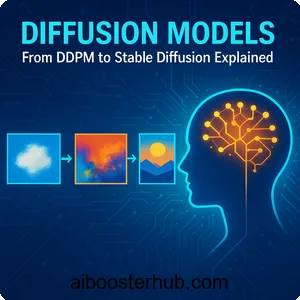
Diffusion Models: From DDPM to Stable Diffusion Explained

Diffusion models have revolutionized the field of generative AI, enabling machines to create stunning images, art, and visual content from simple text descriptions. From the foundational denoising diffusion probabilistic models (DDPM) to the widely-adopted Stable Diffusion, these generative models have transformed how we think about image generation and creative AI applications.

In this comprehensive guide, we’ll explore the mathematical foundations, architectures, and practical implementations of diffusion models. Whether you’re a researcher, developer, or AI enthusiast, understanding these models is crucial for working with modern generative AI systems.

1. Understanding the core concept of diffusion models

What are diffusion models?

Diffusion models are a class of generative models that learn to create data by reversing a gradual noising process. Imagine watching a video of ink slowly dispersing in water—then playing that video backward to see the ink reconstitute itself. That’s essentially what a diffusion model does with images.

The process works in two phases:

• Forward diffusion process: Gradually adds Gaussian noise to data over many timesteps until it becomes pure noise
• Reverse diffusion process: Learns to remove noise step-by-step, reconstructing the original data

This approach differs fundamentally from other generative models like GANs (Generative Adversarial Networks) or VAEs (Variational Autoencoders). While GANs use adversarial training and VAEs compress data into a latent space, diffusion models rely on iterative refinement through noise prediction.

The intuition behind diffusion

Think of a diffusion model as an artist who has forgotten how to draw. To relearn, they practice by taking finished paintings and gradually obscuring them with random brushstrokes. Once they understand this degradation process perfectly, they can work backward—starting with chaos and systematically removing randomness until a coherent image emerges.

This intuition translates into a powerful mathematical framework where the model learns the score (gradient) of the data distribution at different noise levels. By following these gradients, the model can navigate from pure noise back to realistic data samples.

2. DDPM: The foundation of modern diffusion models

Denoising diffusion probabilistic models explained

Denoising diffusion probabilistic models (DDPM) introduced by Ho et al. formalized the diffusion process into a tractable probabilistic framework. DDPM consists of a fixed forward process and a learned reverse process.

The forward process adds noise according to a variance schedule \(\beta_t\) over \(T\) timesteps:

$$ q(x_t | x_{t-1}) = \mathcal{N}(x_t; \sqrt{1-\beta_t} x_{t-1}, \beta_t I) $$

A key insight is that we can sample \(x_t\) directly from \(x_0\) using the reparameterization:

$$ x_t = \sqrt{\bar{\alpha}_t} x_0 + \sqrt{1-\bar{\alpha}_t} \epsilon $$

where \(\bar{\alpha}_t = \prod_{i=1}^{t} (1 – \beta_i),
\quad
\epsilon \sim \mathcal{N}(0, I)\).

The reverse process and noise prediction

The reverse process learns to denoise by predicting the noise that was added:

$$ p_\theta(x_{t-1} | x_t) = \mathcal{N}(x_{t-1}; \mu_\theta(x_t, t), \Sigma_\theta(x_t, t)) $$

Instead of directly predicting \(x_{t-1}\), DDPM trains a neural network \(\epsilon_\theta\) to predict the noise \(\epsilon\), which simplifies the training objective to:

$$ L_{\text{simple}} = \mathbb{E}_{t, x_0, \epsilon}
\left[ \left\| \epsilon – \epsilon_\theta(x_t, t) \right\|^2 \right]$$

This means the model learns to estimate what noise was added at each timestep, allowing it to iteratively remove that noise.

Implementing DDPM in Python

Here’s a simplified implementation of the core DDPM components:

import torch
import torch.nn as nn
import numpy as np

class DDPM:
    def __init__(self, num_timesteps=1000, beta_start=0.0001, beta_end=0.02):
        self.num_timesteps = num_timesteps
        
        # Linear beta schedule
        self.betas = torch.linspace(beta_start, beta_end, num_timesteps)
        self.alphas = 1 - self.betas
        self.alphas_cumprod = torch.cumprod(self.alphas, dim=0)
        
        # Precompute values for forward process
        self.sqrt_alphas_cumprod = torch.sqrt(self.alphas_cumprod)
        self.sqrt_one_minus_alphas_cumprod = torch.sqrt(1 - self.alphas_cumprod)
    
    def forward_diffusion(self, x0, t, noise=None):
        """Add noise to data according to timestep t"""
        if noise is None:
            noise = torch.randn_like(x0)
        
        sqrt_alpha_cumprod_t = self.sqrt_alphas_cumprod[t].reshape(-1, 1, 1, 1)
        sqrt_one_minus_alpha_cumprod_t = self.sqrt_one_minus_alphas_cumprod[t].reshape(-1, 1, 1, 1)
        
        # x_t = sqrt(alpha_bar_t) * x_0 + sqrt(1 - alpha_bar_t) * noise
        return sqrt_alpha_cumprod_t * x0 + sqrt_one_minus_alpha_cumprod_t * noise, noise
    
    def reverse_diffusion(self, model, x_t, t):
        """Remove noise using the trained model"""
        # Predict the noise
        predicted_noise = model(x_t, t)
        
        alpha_t = self.alphas[t].reshape(-1, 1, 1, 1)
        alpha_cumprod_t = self.alphas_cumprod[t].reshape(-1, 1, 1, 1)
        beta_t = self.betas[t].reshape(-1, 1, 1, 1)
        
        # Compute mean of x_{t-1}
        mean = (1 / torch.sqrt(alpha_t)) * (
            x_t - (beta_t / torch.sqrt(1 - alpha_cumprod_t)) * predicted_noise
        )
        
        if t[0] > 0:
            noise = torch.randn_like(x_t)
            variance = beta_t
            return mean + torch.sqrt(variance) * noise
        else:
            return mean

# Training loop example
def train_ddpm(model, dataloader, ddpm, epochs=100, device='cuda'):
    optimizer = torch.optim.Adam(model.parameters(), lr=2e-4)
    
    for epoch in range(epochs):
        for batch in dataloader:
            x0 = batch[0].to(device)
            
            # Sample random timesteps
            t = torch.randint(0, ddpm.num_timesteps, (x0.shape[0],), device=device)
            
            # Add noise
            x_t, noise = ddpm.forward_diffusion(x0, t)
            
            # Predict noise
            predicted_noise = model(x_t, t)
            
            # Compute loss
            loss = nn.MSELoss()(predicted_noise, noise)
            
            optimizer.zero_grad()
            loss.backward()
            optimizer.step()

This implementation shows how DDPM adds noise during training and learns to predict that noise for removal during generation.

3. Score-based models and their connection to diffusion

Understanding score-based generative models

Score-based models provide an alternative perspective on diffusion that illuminates the underlying mathematics. The “score” refers to the gradient of the log probability density:

$$ s_\theta(x, t) = \nabla_x \log p_t(x) $$

This score tells us which direction to move in data space to increase probability density. Score-based models learn this gradient field at different noise levels, then use it to transform noise into data through a process called Langevin dynamics.

The equivalence between score matching and denoising

A remarkable discovery is that denoising and score matching are fundamentally equivalent. When a diffusion model predicts noise (\epsilon_\theta(x_t, t)), it implicitly estimates the score:

$$ s_\theta(x_t, t) = -\frac{\epsilon_\theta(x_t, t)}{\sqrt{1 – \bar{\alpha}_t}} $$

This connection reveals that DDPM performs score matching under the hood. The denoising objective naturally trains the model to estimate probability gradients, which can then guide the reverse diffusion process.

Stochastic differential equations (SDEs)

Score-based models formalize diffusion as a continuous-time stochastic differential equation:

$$ dx = f(x, t)dt + g(t)dw $$

where \(f\) is the drift coefficient, \(g\) is the diffusion coefficient, and (dw) represents Brownian motion. The reverse-time SDE allows sampling:

$$ dx = [f(x, t) – g(t)^2 \nabla_x \log p_t(x)]dt + g(t)d\bar{w} $$

This framework unifies different diffusion formulations and enables flexible sampling strategies through various numerical SDE solvers.

4. Latent diffusion models: Making diffusion efficient

The computational challenge

While DDPM produces impressive results, generating high-resolution images requires hundreds or thousands of denoising steps in pixel space. For a 512×512 image, each step processes over 786,000 values. This computational expense limits practical applications.

Latent diffusion models solve this problem by performing diffusion in a compressed latent space rather than pixel space. This architectural innovation makes high-resolution image generation practical.

How latent diffusion works

The latent diffusion architecture consists of three main components:

1. Autoencoder: A pretrained VAE compresses images into a lower-dimensional latent space
2. Diffusion model: Operates in this compressed space, learning to denoise latent representations
3. Conditioning mechanism: Allows control through text, images, or other modalities

The process looks like:

• Encode image to latent: \(z = \mathcal{E}(x)\)
• Apply diffusion in latent space: \(z_t = \sqrt{\bar{\alpha}_t} z + \sqrt{1-\bar{\alpha}_t} \epsilon\)
• Denoise latent: \(z_0 = \text{DiffusionModel}(z_T)\)
• Decode to image: \(x = \mathcal{D}(z_0)\)

This approach reduces computational requirements by 4-16× while maintaining or improving quality.

Cross-attention for conditioning

Latent diffusion models use cross-attention mechanisms to incorporate conditioning information like text prompts. The denoising U-Net includes cross-attention layers where:

• Query: Comes from the noisy latent representation
• Key and Value: Come from encoded conditioning information (e.g., text embeddings)

This allows the model to attend to relevant parts of the conditioning signal when denoising specific regions of the latent:

class CrossAttentionBlock(nn.Module):
    def __init__(self, dim, context_dim, num_heads=8):
        super().__init__()
        self.num_heads = num_heads
        self.scale = (dim // num_heads) ** -0.5
        
        self.to_q = nn.Linear(dim, dim, bias=False)
        self.to_k = nn.Linear(context_dim, dim, bias=False)
        self.to_v = nn.Linear(context_dim, dim, bias=False)
        self.to_out = nn.Linear(dim, dim)
    
    def forward(self, x, context):
        """
        x: latent features [batch, height*width, dim]
        context: conditioning [batch, seq_len, context_dim]
        """
        batch_size, seq_len, _ = x.shape
        
        # Compute queries from latent, keys and values from context
        q = self.to_q(x)
        k = self.to_k(context)
        v = self.to_v(context)
        
        # Reshape for multi-head attention
        q = q.reshape(batch_size, seq_len, self.num_heads, -1).transpose(1, 2)
        k = k.reshape(batch_size, -1, self.num_heads, -1).transpose(1, 2)
        v = v.reshape(batch_size, -1, self.num_heads, -1).transpose(1, 2)
        
        # Compute attention
        attention_scores = torch.matmul(q, k.transpose(-2, -1)) * self.scale
        attention_probs = torch.softmax(attention_scores, dim=-1)
        
        # Apply attention to values
        out = torch.matmul(attention_probs, v)
        out = out.transpose(1, 2).reshape(batch_size, seq_len, -1)
        
        return self.to_out(out)

5. Stable Diffusion: Architecture and innovations

The Stable Diffusion pipeline

Stable Diffusion represents the culmination of latent diffusion research, combining multiple innovations into a practical, open-source system for text-to-image generation. The complete pipeline includes:

1. Text encoder: CLIP text encoder converts prompts into embeddings
2. Latent diffusion model: U-Net denoises latent representations conditioned on text
3. VAE decoder: Converts final latent back to pixel space
4. Scheduler: Controls the denoising trajectory and sampling algorithm

The architecture processes a text prompt through these stages:

class StableDiffusionPipeline:
    def __init__(self, vae, text_encoder, unet, scheduler):
        self.vae = vae
        self.text_encoder = text_encoder
        self.unet = unet
        self.scheduler = scheduler
    
    def generate(self, prompt, num_inference_steps=50, guidance_scale=7.5):
        # Encode text prompt
        text_embeddings = self.text_encoder(prompt)
        
        # Create unconditional embeddings for classifier-free guidance
        uncond_embeddings = self.text_encoder("")
        
        # Combine for guidance
        text_embeddings = torch.cat([uncond_embeddings, text_embeddings])
        
        # Start from random noise in latent space
        latent = torch.randn((1, 4, 64, 64))
        
        # Set timesteps
        self.scheduler.set_timesteps(num_inference_steps)
        
        # Denoising loop
        for t in self.scheduler.timesteps:
            # Expand latent for classifier-free guidance
            latent_model_input = torch.cat([latent] * 2)
            
            # Predict noise residual
            noise_pred = self.unet(latent_model_input, t, text_embeddings)
            
            # Perform guidance
            noise_pred_uncond, noise_pred_text = noise_pred.chunk(2)
            noise_pred = noise_pred_uncond + guidance_scale * (
                noise_pred_text - noise_pred_uncond
            )
            
            # Compute previous noisy sample
            latent = self.scheduler.step(noise_pred, t, latent)
        
        # Decode latent to image
        image = self.vae.decode(latent)
        return image

Classifier-free guidance

Classifier-free guidance is a crucial technique that allows Stable Diffusion to generate images that closely follow text prompts. During training, the model randomly drops conditioning information, learning both conditional and unconditional distributions.

During inference, the model predicts noise both with and without conditioning, then combines predictions:

$$ \tilde{\epsilon}_\theta(x_t, t, c)
= \epsilon_\theta(x_t, t, \emptyset)
+ w \cdot \left(
\epsilon_\theta(x_t, t, c)
– \epsilon_\theta(x_t, t, \emptyset)
\right) $$

where \(w\) is the guidance scale. Higher values increase prompt adherence but may reduce diversity. Typical values range from 7 to 15.

Sampling algorithms and schedulers

The scheduler determines how the model traverses from noise to data. Different schedulers offer trade-offs between quality and speed:

• DDPM: Original sampling, requires many steps (1000+)
• DDIM: Deterministic sampling, allows fewer steps (50-100)
• DPM-Solver: Fast solver using differential equations (20-25 steps)
• Euler ancestral: Adds controlled noise for diversity

Here’s an example DDIM scheduler implementation:

class DDIMScheduler:
    def __init__(self, num_train_timesteps=1000, beta_start=0.0001, beta_end=0.02):
        self.num_train_timesteps = num_train_timesteps
        self.betas = torch.linspace(beta_start, beta_end, num_train_timesteps)
        self.alphas = 1 - self.betas
        self.alphas_cumprod = torch.cumprod(self.alphas, dim=0)
    
    def set_timesteps(self, num_inference_steps):
        # Create subset of timesteps for faster sampling
        step_ratio = self.num_train_timesteps // num_inference_steps
        self.timesteps = torch.arange(0, self.num_train_timesteps, step_ratio).flip(0)
    
    def step(self, noise_pred, timestep, sample, eta=0.0):
        """Perform one DDIM step"""
        prev_timestep = timestep - self.num_train_timesteps // len(self.timesteps)
        
        alpha_prod_t = self.alphas_cumprod[timestep]
        alpha_prod_t_prev = self.alphas_cumprod[prev_timestep] if prev_timestep >= 0 else 1.0
        
        # Predict x_0
        pred_original_sample = (
            sample - torch.sqrt(1 - alpha_prod_t) * noise_pred
        ) / torch.sqrt(alpha_prod_t)
        
        # Compute variance
        variance = (1 - alpha_prod_t_prev) / (1 - alpha_prod_t) * (1 - alpha_prod_t / alpha_prod_t_prev)
        std_dev_t = eta * torch.sqrt(variance)
        
        # Compute direction to x_t
        pred_sample_direction = torch.sqrt(1 - alpha_prod_t_prev - std_dev_t**2) * noise_pred
        
        # Compute x_{t-1}
        prev_sample = torch.sqrt(alpha_prod_t_prev) * pred_original_sample + pred_sample_direction
        
        if eta > 0:
            noise = torch.randn_like(sample)
            prev_sample += std_dev_t * noise
        
        return prev_sample

6. Advanced techniques and applications

Image-to-image and inpainting

Diffusion models excel at image-to-image translation and inpainting by starting from partially noised images rather than pure noise. For image-to-image generation:

1. Encode the input image to latent space
2. Add noise according to a strength parameter (e.g., 50% noise)
3. Denoise using the text prompt as guidance
4. Decode the result

This allows for controlled modifications while preserving structure:

def img2img(pipeline, init_image, prompt, strength=0.8, num_steps=50):
    # Encode initial image
    latent = pipeline.vae.encode(init_image)
    
    # Determine starting timestep based on strength
    start_step = int(num_steps * strength)
    start_timestep = pipeline.scheduler.timesteps[start_step]
    
    # Add noise to latent
    noise = torch.randn_like(latent)
    latent = pipeline.scheduler.add_noise(latent, noise, start_timestep)
    
    # Denoise from this point
    for t in pipeline.scheduler.timesteps[start_step:]:
        # Standard denoising step
        latent = pipeline.denoise_step(latent, t, prompt)
    
    return pipeline.vae.decode(latent)

ControlNet and spatial conditioning

ControlNet adds precise spatial control to diffusion models by processing additional input conditions (edges, poses, depth maps) through a parallel network architecture. This enables applications like:

• Pose-guided character generation
• Depth-aware scene composition
• Edge-guided image synthesis

The ControlNet copies the U-Net weights and processes control images alongside the main diffusion process, adding its outputs to the main network through zero-initialized connections.

Fine-tuning and personalization

Several techniques enable customizing Stable Diffusion for specific subjects or styles:

• DreamBooth: Fine-tunes the entire model on 3-5 images with a unique identifier
• Textual Inversion: Learns new token embeddings while keeping the model frozen
• LoRA: Learns low-rank adaptations of attention weights, requiring minimal storage

These methods make personalized image generation accessible without massive computational resources.

7. Practical considerations and future directions

Training considerations

Training diffusion models requires careful attention to several factors:

• Batch size and resolution: Larger batches stabilize training but require more memory. Start at 64×64 or 128×128 resolution and increase gradually.
• Learning rate scheduling: Constant or cosine schedules work well. Typical values: 1e-4 to 2e-4.
• Noise schedule: Linear schedules work for DDPM, but cosine schedules often perform better for high-resolution images.
• EMA weights: Maintaining exponential moving averages of model weights improves sample quality.

Optimization and efficiency

Several techniques accelerate diffusion model inference:

• Reduced precision: Float16 or bfloat16 reduces memory and increases speed
• Flash attention: Optimized attention implementations reduce computational cost
• Model distillation: Trains smaller models to mimic larger ones in fewer steps
• Latent consistency models: Recent approaches enable single-step generation

Challenges and limitations

Despite their success, diffusion models face ongoing challenges:

• Text-image alignment: Models sometimes struggle with complex spatial relationships or counting
• Bias and fairness: Training data biases can propagate to generated images
• Computational cost: Generation still requires significant resources
• Fine details: Very small or intricate details may appear inconsistent

Emerging research directions

The field continues to evolve rapidly with exciting developments:

• Video diffusion: Extending models to generate coherent video sequences
• 3D generation: Creating three-dimensional objects and scenes
• Multi-modal fusion: Combining text, audio, and image conditioning
• Faster sampling: Reducing inference steps while maintaining quality
• Disentangled control: Separating style, content, and composition

8. Knowledge Check