Attention Mechanisms: CBAM and Non-Local Neural Networks

The evolution of convolutional neural networks has been marked by continuous improvements in how models process and understand visual information. Among the most impactful innovations are attention mechanisms, which enable networks to focus on the most relevant features while suppressing less important information. Two particularly influential approaches—CBAM (Convolutional Block Attention Module) and Non-Local Neural Networks—have revolutionized how we build neural network architectures for computer vision tasks.

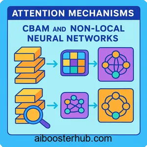
Attention mechanisms in CNN architectures address a fundamental challenge: not all features are equally important for making predictions. By learning to emphasize critical information and ignore noise, these mechanisms significantly improve model performance without massive increases in computational cost. Understanding how CBAM and non-local neural networks implement attention provides crucial insights for anyone working with deep learning in computer vision.

Content

1. Understanding attention mechanisms in neural networks

Attention mechanisms draw inspiration from human visual perception. When you look at a crowded scene, your brain doesn’t process every pixel with equal importance—it focuses on salient objects and regions. Similarly, attention in CNN architectures allows networks to dynamically weight different features based on their relevance to the task at hand.

The evolution from basic CNNs to attention-based models

Traditional convolutional neural networks process images through a series of convolution operations, pooling layers, and fully connected layers. While powerful, these networks treat all spatial locations and channels with equal importance during feature extraction. This uniform treatment can be suboptimal when certain regions or feature maps contain more discriminative information than others.

The introduction of attention mechanisms marked a paradigm shift. Instead of relying solely on the hierarchical feature learning of convolutions, attention-based models explicitly learn to highlight important features. This is achieved through learnable attention weights that modulate the original features, creating a more adaptive and context-aware representation.

Types of attention in computer vision

Attention mechanisms in computer vision typically fall into three categories: spatial attention, channel attention, and self-attention. Spatial attention focuses on “where” to pay attention in the spatial dimensions of the feature map. It learns to assign importance to different spatial locations, effectively creating a spatial attention map that highlights regions of interest.

Channel attention, on the other hand, emphasizes “what” to pay attention to among different feature channels. Since each channel in a CNN typically responds to different semantic features (edges, textures, object parts), channel attention helps the network select the most informative channels for the task.

Self-attention, popularized by non-local neural networks, captures long-range dependencies by computing relationships between all positions in the feature map.

2. CBAM: Convolutional block attention module architecture

CBAM represents an elegant solution to incorporating both spatial and channel attention into convolutional neural networks. The beauty of CBAM lies in its simplicity and effectiveness—it’s a lightweight module that can be seamlessly integrated into any CNN architecture with minimal computational overhead.

Channel attention mechanism

The channel attention module in CBAM addresses the question of “what” is meaningful in the feature maps. Given an input feature map with dimensions $H \times W \times C$ (height, width, channels), the channel attention module first applies both average pooling and max pooling operations across the spatial dimensions, producing two context descriptors of size $1 \times 1 \times C$.

These descriptors are then fed through a shared multi-layer perceptron (MLP) network consisting of two fully connected layers. The first layer reduces the dimensionality by a reduction ratio $r$ (typically 16), applies a ReLU activation, and the second layer restores the original channel dimension. Mathematically, the channel attention $M_c$ is computed as:

$$M_c(F) = \sigma(MLP(AvgPool(F)) + MLP(MaxPool(F)))$$

where $\sigma$ represents the sigmoid activation function, and $F$ is the input feature map. The resulting channel attention map is then element-wise multiplied with the input feature map to produce a channel-refined output.

Spatial attention mechanism

Following channel attention, CBAM applies spatial attention to emphasize informative spatial locations. The spatial attention module takes the channel-refined feature map and applies average pooling and max pooling operations along the channel dimension, creating two 2D maps of size $H \times W \times 1$.

These two maps are concatenated and passed through a convolutional layer with a $7 \times 7$ kernel (though kernel size can vary), followed by a sigmoid activation. The spatial attention $M_s$ is formulated as:

$$M_s(F’) = \sigma(f^{7\times7}([AvgPool(F’); MaxPool(F’)]))$$

where $F$ is the channel-refined feature map, $f^{7\times7}$ represents the convolution operation, and $[;]$ denotes concatenation. The resulting spatial attention map highlights regions that should receive more focus.

Sequential channel-spatial attention

The key insight of CBAM is the sequential application of channel and spatial attention. By first refining features along the channel dimension and then along the spatial dimension, CBAM efficiently captures both “what” and “where” to focus on. The complete CBAM module can be expressed as:

$$F’ = M_c(F) \otimes F$$ $$F” = M_s(F’) \otimes F’$$

where $\otimes$ denotes element-wise multiplication. This sequential approach has been empirically shown to outperform parallel attention mechanisms or single-dimension attention.

Implementation example

Here’s a practical implementation of CBAM in Python using PyTorch:

import torch
import torch.nn as nn

class ChannelAttention(nn.Module):
    def __init__(self, in_channels, reduction_ratio=16):
        super(ChannelAttention, self).__init__()
        self.avg_pool = nn.AdaptiveAvgPool2d(1)
        self.max_pool = nn.AdaptiveMaxPool2d(1)
        
        self.mlp = nn.Sequential(
            nn.Linear(in_channels, in_channels // reduction_ratio, bias=False),
            nn.ReLU(inplace=True),
            nn.Linear(in_channels // reduction_ratio, in_channels, bias=False)
        )
        self.sigmoid = nn.Sigmoid()
    
    def forward(self, x):
        b, c, h, w = x.size()
        
        # Average pooling path
        avg_pool = self.avg_pool(x).view(b, c)
        avg_out = self.mlp(avg_pool)
        
        # Max pooling path
        max_pool = self.max_pool(x).view(b, c)
        max_out = self.mlp(max_pool)
        
        # Combine and apply sigmoid
        out = self.sigmoid(avg_out + max_out).view(b, c, 1, 1)
        return out * x

class SpatialAttention(nn.Module):
    def __init__(self, kernel_size=7):
        super(SpatialAttention, self).__init__()
        padding = (kernel_size - 1) // 2
        self.conv = nn.Conv2d(2, 1, kernel_size, padding=padding, bias=False)
        self.sigmoid = nn.Sigmoid()
    
    def forward(self, x):
        # Generate channel-wise statistics
        avg_out = torch.mean(x, dim=1, keepdim=True)
        max_out, _ = torch.max(x, dim=1, keepdim=True)
        
        # Concatenate and convolve
        combined = torch.cat([avg_out, max_out], dim=1)
        attention = self.sigmoid(self.conv(combined))
        
        return attention * x

class CBAM(nn.Module):
    def __init__(self, in_channels, reduction_ratio=16, kernel_size=7):
        super(CBAM, self).__init__()
        self.channel_attention = ChannelAttention(in_channels, reduction_ratio)
        self.spatial_attention = SpatialAttention(kernel_size)
    
    def forward(self, x):
        x = self.channel_attention(x)
        x = self.spatial_attention(x)
        return x

# Example usage
if __name__ == "__main__":
    # Create a sample input tensor (batch_size=2, channels=64, height=32, width=32)
    input_tensor = torch.randn(2, 64, 32, 32)
    
    # Initialize CBAM module
    cbam = CBAM(in_channels=64)
    
    # Forward pass
    output = cbam(input_tensor)
    print(f"Input shape: {input_tensor.shape}")
    print(f"Output shape: {output.shape}")

This implementation demonstrates how CBAM can be easily integrated into existing architectures. The module is designed to be placed after convolutional blocks, where it refines the learned features before passing them to the next layer.

3. Non-local neural networks and self-attention

While CBAM focuses on channel and spatial attention within local regions, non-local neural networks take a different approach by capturing long-range dependencies through self-attention. This paradigm shift allows the network to model relationships between distant spatial locations, overcoming the limited receptive field constraints of traditional convolutions.

The limitation of local operations

Standard convolutional operations are inherently local—each output position is computed from a small neighborhood of input positions defined by the kernel size. While stacking multiple convolutional layers can expand the receptive field, building long-range dependencies requires many layers, making the network deep and potentially inefficient.

This locality constraint becomes particularly problematic for tasks requiring global context understanding. For example, recognizing that a small object is a “tennis ball” might require understanding that it appears in a scene with a tennis court and a person holding a racket—relationships that span the entire image.

Non-local operations formulation

Non-local neural networks introduce non-local blocks that compute the response at a position as a weighted sum of features at all positions. The operation can be formulated as:

$$y_i = \frac{1}{C(x)} \sum_{\forall j} f(x_i, x_j) g(x_j)$$

where $x_i$ represents the input feature at position $i$, $y_i$ is the output at the same position, $f$ is a pairwise function computing the relationship between positions $i$ and $j$, $g$ is a transformation of the input, and $C(x)$ is a normalization factor.

Different instantiations of non-local blocks

The pairwise function $f$ can take various forms, each offering different properties. The Gaussian instantiation uses:

$$f(x_i, x_j) = e^{x_i^T x_j}$$

This measures similarity through a dot product in the embedded space. The embedded Gaussian variant first transforms the features through learned embeddings $\theta$ and $\phi$:

$$f(x_i, x_j) = e^{\theta(x_i)^T \phi(x_j)}$$

After softmax normalization, this formulation becomes equivalent to the self-attention mechanism used in Transformer architectures. The dot product version simplifies this further:

$$f(x_i, x_j) = \theta(x_i)^T \phi(x_j)$$

In practice, the embedded Gaussian formulation has shown excellent performance across various tasks and is the most commonly used variant.

Implementation of non-local blocks

Here’s how to implement a non-local block in PyTorch:

import torch
import torch.nn as nn
import torch.nn.functional as F

class NonLocalBlock(nn.Module):
    def __init__(self, in_channels, inter_channels=None, sub_sample=True):
        super(NonLocalBlock, self).__init__()
        
        self.in_channels = in_channels
        self.inter_channels = inter_channels or in_channels // 2
        
        # Define transformation functions
        self.theta = nn.Conv2d(in_channels, self.inter_channels, 
                               kernel_size=1, stride=1, padding=0)
        self.phi = nn.Conv2d(in_channels, self.inter_channels, 
                             kernel_size=1, stride=1, padding=0)
        self.g = nn.Conv2d(in_channels, self.inter_channels, 
                           kernel_size=1, stride=1, padding=0)
        
        # Output transformation
        self.W = nn.Sequential(
            nn.Conv2d(self.inter_channels, in_channels, 
                     kernel_size=1, stride=1, padding=0),
            nn.BatchNorm2d(in_channels)
        )
        
        # Initialize W to output zeros initially (residual connection)
        nn.init.constant_(self.W[1].weight, 0)
        nn.init.constant_(self.W[1].bias, 0)
        
        # Optional sub-sampling for efficiency
        self.sub_sample = sub_sample
        if sub_sample:
            self.phi = nn.Sequential(
                self.phi,
                nn.MaxPool2d(kernel_size=2)
            )
            self.g = nn.Sequential(
                self.g,
                nn.MaxPool2d(kernel_size=2)
            )
    
    def forward(self, x):
        batch_size, C, H, W = x.size()
        
        # Compute theta (query)
        theta_x = self.theta(x).view(batch_size, self.inter_channels, -1)
        theta_x = theta_x.permute(0, 2, 1)  # [B, HW, C']
        
        # Compute phi (key)
        phi_x = self.phi(x).view(batch_size, self.inter_channels, -1)  # [B, C', HW]
        
        # Compute attention map
        attention = torch.matmul(theta_x, phi_x)  # [B, HW, HW]
        attention = F.softmax(attention, dim=-1)
        
        # Compute g (value)
        g_x = self.g(x).view(batch_size, self.inter_channels, -1)
        g_x = g_x.permute(0, 2, 1)  # [B, HW, C']
        
        # Apply attention
        y = torch.matmul(attention, g_x)  # [B, HW, C']
        y = y.permute(0, 2, 1).contiguous()
        y = y.view(batch_size, self.inter_channels, H, W)
        
        # Transform and add residual
        W_y = self.W(y)
        output = W_y + x
        
        return output

# Example usage with visualization
if __name__ == "__main__":
    # Create input tensor
    input_tensor = torch.randn(2, 256, 28, 28)
    
    # Initialize non-local block
    non_local = NonLocalBlock(in_channels=256, inter_channels=128)
    
    # Forward pass
    output = non_local(input_tensor)
    
    print(f"Input shape: {input_tensor.shape}")
    print(f"Output shape: {output.shape}")
    print(f"Attention map size: {28*28} x {28*28} (for each sample)")

The non-local block can be inserted at various depths in a neural network architecture. It’s particularly effective when placed in the middle or later stages where the spatial resolution is smaller, making the attention computation more tractable.

4. Comparing CBAM and non-local approaches

Both CBAM convolutional block attention module and non-local neural networks enhance traditional CNN architectures through attention mechanisms, but they differ significantly in their approaches, computational requirements, and use cases.

Computational complexity analysis

CBAM is designed to be lightweight and efficient. The channel attention module involves global pooling operations and a small MLP, while spatial attention uses a single convolutional layer. For a feature map of size $H \times W \times C$, the computational cost is approximately $O(C^2/r + HWk^2)$, where $r$ is the reduction ratio and $k$ is the spatial convolution kernel size. This makes CBAM extremely parameter-efficient, adding minimal overhead to the base network.

Non-local blocks, in contrast, compute pairwise relationships between all spatial positions, resulting in $O((HW)^2 C)$ complexity. The attention matrix alone requires $O((HW)^2)$ memory, which can become prohibitive for high-resolution feature maps. To address this, non-local blocks are typically applied to downsampled feature maps and may use subsampling strategies within the block itself.

Attention scope and receptive field

CBAM operates on local statistics—channel attention aggregates information across the entire spatial extent but treats each channel independently, while spatial attention focuses on local spatial patterns within the convolution kernel size. This makes CBAM excellent at highlighting important channels and spatial regions based on global context, but it doesn’t explicitly model relationships between distant locations.

Non-local neural networks excel at capturing long-range dependencies. Every position can directly attend to every other position, enabling the network to understand global context without requiring deep stacking of layers. This is particularly valuable for tasks like video understanding, where temporal relationships between distant frames matter, or for modeling non-local spatial relationships in images.

Integration flexibility

CBAM’s modular design allows it to be inserted after any convolutional block in existing architectures with minimal modifications. You can add CBAM to ResNet, VGG, or any custom CNN architecture by simply placing the module after convolutional blocks. The sequential channel-spatial design ensures compatibility with various feature map sizes.

Non-local blocks also integrate into existing architectures but require more careful consideration. Due to their computational cost, they’re typically added sparingly—often just one or two blocks in the entire network. The residual connection design (output = input + transformed_features) ensures that the network can gracefully learn to use or ignore the non-local information.

Performance characteristics

In practice, CBAM provides consistent improvements across various tasks with minimal computational overhead—typically 1-2% accuracy gains with less than 1% increase in parameters. It’s particularly effective for object detection, image classification, and semantic segmentation where identifying important channels and spatial regions is crucial.

Non-local blocks shine in scenarios requiring long-range dependency modeling. They’ve shown remarkable success in video classification, action recognition, and instance segmentation tasks. The performance gains are often more substantial but come with higher computational costs, making them most suitable for applications where the accuracy improvement justifies the additional computation.

5. Practical applications and use cases

Understanding the theoretical foundations of attention mechanisms is only the first step—their true value emerges in real-world applications. Both CBAM and non-local neural networks have found success across diverse computer vision tasks.

Object detection and recognition

In object detection frameworks like Faster R-CNN, YOLO, or RetinaNet, attention mechanisms help the network focus on regions containing objects while suppressing background noise. CBAM can be integrated into the backbone network (such as ResNet or MobileNet) to improve feature extraction quality. The channel attention helps emphasize feature maps that respond strongly to object-specific patterns, while spatial attention highlights object locations.

For example, when detecting small objects in cluttered scenes, spatial attention in CBAM can amplify features around tiny objects that might otherwise be overwhelmed by background features. This is particularly valuable in applications like autonomous driving, where detecting small but critical objects (pedestrians, traffic signs) at a distance is essential.

Image segmentation tasks

Semantic segmentation requires dense predictions—assigning a class label to every pixel in the image. Non-local neural networks have proven particularly effective here because understanding the class of one pixel often depends on global scene context. For instance, a blue region might be “sky” or “water” depending on what else appears in the image.

By incorporating non-local blocks in segmentation architectures like DeepLab or PSPNet, the network can model long-range contextual relationships. A pixel’s segmentation benefits from attending to all other pixels, enabling the network to understand scene layout and object co-occurrence patterns. This leads to more consistent segmentations with fewer isolated misclassifications.

Video understanding and temporal modeling

Video analysis presents unique challenges—models must understand not just spatial patterns but also temporal dynamics. Non-local neural networks naturally extend to video by treating time as an additional dimension. A non-local block can compute attention across space-time, allowing the network to model relationships between frames separated by significant time intervals.

This capability is crucial for action recognition, where understanding an action might require relating movements across many frames. For example, recognizing “basketball dunk” requires linking the player’s jumping motion with the ball’s trajectory and the moment of scoring—events that may span dozens of frames. Non-local blocks enable this temporal reasoning without requiring extremely deep temporal convolutions.

Medical image analysis

Medical imaging applications benefit significantly from attention mechanisms. In radiology, for instance, pathological regions might be small relative to the entire image, and their identification often requires understanding anatomical context. CBAM helps by learning to emphasize feature channels and spatial locations that correlate with diagnostic patterns.

Non-local blocks are valuable in medical imaging for capturing long-range anatomical relationships. In whole-slide pathology images, the diagnosis might depend on patterns distributed across large tissue areas. Non-local attention allows the network to integrate information across distant tissue regions, improving diagnostic accuracy.

Practical implementation considerations

Here’s an example of integrating CBAM into a ResNet-style architecture for image classification:

import torch
import torch.nn as nn

class ResBlockWithCBAM(nn.Module):
    def __init__(self, in_channels, out_channels, stride=1):
        super(ResBlockWithCBAM, self).__init__()
        
        # Standard residual block components
        self.conv1 = nn.Conv2d(in_channels, out_channels, 
                               kernel_size=3, stride=stride, padding=1, bias=False)
        self.bn1 = nn.BatchNorm2d(out_channels)
        self.relu = nn.ReLU(inplace=True)
        
        self.conv2 = nn.Conv2d(out_channels, out_channels, 
                               kernel_size=3, stride=1, padding=1, bias=False)
        self.bn2 = nn.BatchNorm2d(out_channels)
        
        # CBAM attention module
        self.cbam = CBAM(out_channels)
        
        # Shortcut connection
        self.shortcut = nn.Sequential()
        if stride != 1 or in_channels != out_channels:
            self.shortcut = nn.Sequential(
                nn.Conv2d(in_channels, out_channels, 
                         kernel_size=1, stride=stride, bias=False),
                nn.BatchNorm2d(out_channels)
            )
    
    def forward(self, x):
        identity = self.shortcut(x)
        
        out = self.conv1(x)
        out = self.bn1(out)
        out = self.relu(out)
        
        out = self.conv2(out)
        out = self.bn2(out)
        
        # Apply CBAM attention
        out = self.cbam(out)
        
        out += identity
        out = self.relu(out)
        
        return out

class AttentionResNet(nn.Module):
    def __init__(self, num_classes=1000):
        super(AttentionResNet, self).__init__()
        
        self.conv1 = nn.Conv2d(3, 64, kernel_size=7, stride=2, padding=3, bias=False)
        self.bn1 = nn.BatchNorm2d(64)
        self.relu = nn.ReLU(inplace=True)
        self.maxpool = nn.MaxPool2d(kernel_size=3, stride=2, padding=1)
        
        # Residual blocks with CBAM
        self.layer1 = self._make_layer(64, 64, num_blocks=2)
        self.layer2 = self._make_layer(64, 128, num_blocks=2, stride=2)
        self.layer3 = self._make_layer(128, 256, num_blocks=2, stride=2)
        self.layer4 = self._make_layer(256, 512, num_blocks=2, stride=2)
        
        self.avgpool = nn.AdaptiveAvgPool2d((1, 1))
        self.fc = nn.Linear(512, num_classes)
    
    def _make_layer(self, in_channels, out_channels, num_blocks, stride=1):
        layers = []
        layers.append(ResBlockWithCBAM(in_channels, out_channels, stride))
        for _ in range(1, num_blocks):
            layers.append(ResBlockWithCBAM(out_channels, out_channels))
        return nn.Sequential(*layers)
    
    def forward(self, x):
        x = self.conv1(x)
        x = self.bn1(x)
        x = self.relu(x)
        x = self.maxpool(x)
        
        x = self.layer1(x)
        x = self.layer2(x)
        x = self.layer3(x)
        x = self.layer4(x)
        
        x = self.avgpool(x)
        x = torch.flatten(x, 1)
        x = self.fc(x)
        
        return x

# Training example
def train_model():
    device = torch.device("cuda" if torch.cuda.is_available() else "cpu")
    model = AttentionResNet(num_classes=10).to(device)
    criterion = nn.CrossEntropyLoss()
    optimizer = torch.optim.Adam(model.parameters(), lr=0.001)
    
    # Dummy training loop
    for epoch in range(5):
        model.train()
        # Simulate batch of images
        inputs = torch.randn(16, 3, 224, 224).to(device)
        labels = torch.randint(0, 10, (16,)).to(device)
        
        optimizer.zero_grad()
        outputs = model(inputs)
        loss = criterion(outputs, labels)
        loss.backward()
        optimizer.step()
        
        print(f"Epoch {epoch+1}, Loss: {loss.item():.4f}")

if __name__ == "__main__":
    print("Initializing Attention-based ResNet...")
    model = AttentionResNet(num_classes=10)
    print(f"Total parameters: {sum(p.numel() for p in model.parameters()):,}")

This implementation demonstrates how seamlessly CBAM integrates into standard architectures, requiring minimal code changes while providing attention benefits throughout the network.

6. Hybrid approaches and future directions

As attention mechanisms mature, researchers increasingly explore hybrid approaches that combine the strengths of different attention types. The complementary nature of CBAM and non-local neural networks suggests that combining them could yield even better results.

Combining local and global attention

Some architectures use CBAM for efficient local attention refinement while strategically placing non-local blocks to capture global dependencies. For instance, you might apply CBAM after every residual block for consistent feature refinement, while adding one or two non-local blocks in the deeper layers where the spatial resolution is manageable and global context is most valuable.

This hybrid approach balances computational efficiency with modeling capacity. CBAM provides consistent improvements throughout the network with minimal cost, while non-local blocks add global reasoning capabilities at critical points. The combination often outperforms using either mechanism alone.

Efficient attention mechanisms

The computational cost of non-local operations has motivated research into more efficient self-attention variants. Techniques like local self-attention (restricting attention to local neighborhoods), axial attention (computing attention separately along height and width), and efficient attention (using kernel approximations) reduce complexity while maintaining much of the benefit of full non-local attention.

These efficient variants make self-attention more practical for high-resolution inputs and resource-constrained deployments. For example, axial attention reduces complexity from $O((HW)^2)$ to $O(HW(H+W))$, making it feasible to apply attention to larger feature maps.

Attention in modern architectures

Recent neural network architecture trends show increasing integration of attention mechanisms. Vision Transformers (ViT) go further by replacing convolutions entirely with self-attention, demonstrating that attention can serve as a fundamental building block rather than just an add-on module. However, hybrid architectures that combine convolutional inductive biases with attention mechanisms often achieve the best trade-offs between performance, data efficiency, and computational cost.

The success of attention in vision has also inspired cross-domain applications. Attention mechanisms originally developed for vision (like CBAM) have been adapted for time-series analysis, audio processing, and even graph neural networks, demonstrating the universality of the attention concept.

Interpretability and visualization

One often-overlooked benefit of attention mechanisms is improved model interpretability. The attention maps learned by CBAM and non-local blocks provide insights into what the network considers important. Visualizing channel attention reveals which feature channels are emphasized for different inputs, while spatial attention maps highlight regions the network focuses on for making predictions.

For non-local blocks, the attention matrix shows which spatial locations influence each other, revealing the global relationships the network has learned. These visualizations can help practitioners understand model behavior, debug failures, and build trust in AI systems—particularly important for applications like medical diagnosis or autonomous driving where understanding model reasoning is crucial.

7. Conclusion

Attention mechanisms have fundamentally transformed how we design and understand convolutional neural networks. CBAM and non-local neural networks represent two powerful but distinct approaches to incorporating attention into CNN architectures. CBAM offers an efficient, modular solution that refines features through sequential channel and spatial attention, making it ideal for resource-constrained applications where consistent performance improvements are needed. Non-local neural networks provide sophisticated global context modeling through self-attention, excelling in tasks that require understanding long-range dependencies despite higher computational costs.

The choice between these approaches—or their combination—depends on your specific application requirements, computational constraints, and the nature of your data. As attention mechanisms continue to evolve, they remain essential tools in the modern computer vision practitioner’s toolkit, bridging the gap between biological visual perception and artificial neural networks.

Explore more: