Cooperative Multi-Agent Reinforcement Learning Guide
Multi-agent reinforcement learning (MARL) represents one of the most exciting frontiers in artificial intelligence, where multiple agents learn to work together to achieve common goals. Unlike traditional single-agent reinforcement learning, cooperative MARL introduces unique challenges and opportunities that mirror real-world scenarios where collaboration is essential. From autonomous vehicle fleets coordinating traffic flow to robotic teams assembling complex products, the applications of cooperative reinforcement learning are transforming how we approach multi-task scenarios.
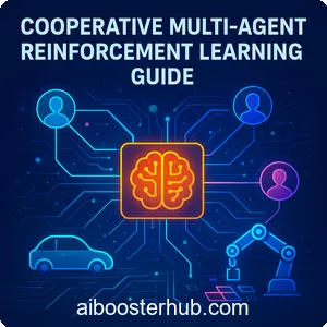
This comprehensive guide explores the foundations of multi-agent reinforcement learning, diving deep into cooperative strategies, algorithmic approaches, and practical implementations that make MARL a cornerstone of modern AI systems.
Content
Toggle1. Understanding multi-agent reinforcement learning fundamentals
What is multi-agent reinforcement learning?
Multi-agent reinforcement learning extends the classic reinforcement learning paradigm to environments where multiple agents interact simultaneously. While single-agent RL focuses on one learner optimizing its policy in a static environment, MARL deals with the complexity of multiple learners whose actions affect each other’s experiences and outcomes.
In a multi-agent system, each agent maintains its own policy \( \pi_i \) and learns through interactions with both the environment and other agents. The key distinction lies in the non-stationary nature of the environment from each agent’s perspective—as other agents learn and adapt their policies, the environment dynamics change continuously.
Cooperative vs competitive MARL
MARL scenarios typically fall into three categories:
Cooperative settings require all agents to work toward a shared objective. Examples include robot swarms performing search and rescue operations or distributed sensor networks optimizing coverage. In these scenarios, agents must learn to coordinate their actions to maximize a global reward signal.
Competitive settings pit agents against each other, similar to zero-sum games where one agent’s gain is another’s loss. Classic examples include game-playing AI systems.
Mixed settings combine both cooperative and competitive elements, such as team-based games where agents cooperate within teams while competing against opposing teams.
This guide focuses primarily on cooperative multi-agent reinforcement learning, where the collective success of the team outweighs individual performance.
Key challenges in MARL
Several fundamental challenges distinguish MARL from single-agent RL:
Non-stationarity: As agents learn simultaneously, the environment appears non-stationary from each agent’s perspective. An optimal policy at one timestep may become suboptimal as teammates adapt their strategies.
Credit assignment: When multiple agents contribute to a team reward, determining each agent’s individual contribution becomes difficult. This problem intensifies in scenarios with delayed rewards and long action sequences.
Scalability: As the number of agents increases, the joint action space grows exponentially, making learning computationally prohibitive. A system with \( n \) agents, each with \( k \) possible actions, has \( k^n \) joint actions.
Partial observability: In many realistic scenarios, agents can only observe local information, requiring them to make decisions based on incomplete knowledge of the global state.
2. Mathematical foundations of cooperative MARL
Markov games and stochastic games
Cooperative MARL is typically formalized as a Markov game, also called a stochastic game. A Markov game for \( n \) agents is defined by the tuple \( \langle \mathcal{S}, \mathcal{A}_1, \ldots, \mathcal{A}_n, \mathcal{P}, \mathcal{R}_1, \ldots, \mathcal{R}_n, \gamma \rangle \), where:
- \( \mathcal{S} \) is the set of states
- \( \mathcal{A}_i \) is the action space for agent \( i \)
- \( \mathcal{P}: \mathcal{S} \times \mathcal{A}_1 \times \cdots \times \mathcal{A}_n \rightarrow \Delta(\mathcal{S}) \) is the state transition function
- \( \mathcal{R}_i: \mathcal{S} \times \mathcal{A}_1 \times \cdots \times \mathcal{A}_n \rightarrow \mathbb{R} \) is the reward function for agent \( i \)
- \( \gamma \in [0, 1) \) is the discount factor
In cooperative settings, all agents share the same reward function: \( \mathcal{R}_1 = \mathcal{R}_2 = \cdots = \mathcal{R}_n = \mathcal{R} \). This transforms the problem into optimizing a shared objective.
Joint action-value functions
The joint action-value function represents the expected return when all agents take specific actions in a given state:
$$ Q(\mathbf{s}, \mathbf{a}) = \mathbb{E}\left[\sum_{t=0}^{\infty} \gamma^t r_{t+1} \mid \mathbf{s}_0 = \mathbf{s}, \mathbf{a}_0 = \mathbf{a}\right] $$
where \( \mathbf{a} = (a_1, a_2, \ldots, a_n) \) represents the joint action of all agents. The goal of cooperative reinforcement learning is to find a joint policy \( \boldsymbol{\pi} = (\pi_1, \pi_2, \ldots, \pi_n) \) that maximizes this expected return.
Individual-global-max (IGM) principle
A crucial concept in cooperative MARL is the IGM principle, which ensures that the optimal global action can be decomposed into individual optimal actions. Formally, if each agent ( i ) selects \( a_i = \arg\max_{a_i’} Q_i(s, a_i’) \), then the joint action \( \mathbf{a} = (a_1, \ldots, a_n) \) satisfies:
$$ \mathbf{a} = \arg\max_{\mathbf{a}’} Q_{tot}(\mathbf{s}, \mathbf{a}’) $$
This principle enables decentralized execution where agents can select actions independently based on local information while still achieving globally optimal behavior.
3. Core algorithms for cooperative multi-agent reinforcement learning
Independent Q-learning (IQL)
The simplest approach to MARL is Independent Q-learning, where each agent learns its own Q-function independently, treating other agents as part of the environment. Each agent \( i \) updates its Q-values using standard Q-learning:
$$ Q_i(s, a_i) \leftarrow Q_i(s, a_i) + \alpha\left[r + \gamma \max_{a_i’} Q_i(s’, a_i’) – Q_i(s, a_i)\right] $$
Here’s a simple implementation:
import numpy as np

class IndependentQLearning:
    def __init__(self, n_agents, n_states, n_actions, alpha=0.1, gamma=0.99, epsilon=0.1):
        self.n_agents = n_agents
        self.n_states = n_states
        self.n_actions = n_actions
        self.alpha = alpha
        self.gamma = gamma
        self.epsilon = epsilon

        # Initialize Q-tables for each agent
        self.q_tables = [np.zeros((n_states, n_actions)) for _ in range(n_agents)]

    def select_actions(self, state):
        """Select actions for all agents using epsilon-greedy policy"""
        actions = []
        for agent_id in range(self.n_agents):
            if np.random.random() < self.epsilon:
                action = np.random.randint(self.n_actions)
            else:
                action = np.argmax(self.q_tables[agent_id][state])
            actions.append(action)
        return actions

    def update(self, state, actions, reward, next_state):
        """Update Q-values for all agents"""
        for agent_id in range(self.n_agents):
            current_q = self.q_tables[agent_id][state, actions[agent_id]]
            max_next_q = np.max(self.q_tables[agent_id][next_state])
            new_q = current_q + self.alpha * (reward + self.gamma * max_next_q - current_q)
            self.q_tables[agent_id][state, actions[agent_id]] = new_q

# Example usage
marl_system = IndependentQLearning(n_agents=3, n_states=10, n_actions=4)
state = 0
actions = marl_system.select_actions(state)
# After environment step: reward, next_state
marl_system.update(state, actions, reward=1.0, next_state=1)
While IQL is simple and scalable, it suffers from non-stationarity issues since each agent’s learning affects others’ experiences.
Value decomposition networks (VDN)
VDN addresses the credit assignment problem by decomposing the team value function into individual agent value functions. The key insight is that the global Q-value can be represented as a sum:
$$ Q_{tot}(\mathbf{s}, \mathbf{a}) = \sum_{i=1}^{n} Q_i(s, a_i) $$
This additive decomposition ensures the IGM principle holds. Here’s a PyTorch-style implementation:
import numpy as np

class VDN:
    def __init__(self, n_agents, state_dim, action_dim, hidden_dim=64):
        self.n_agents = n_agents
        self.state_dim = state_dim
        self.action_dim = action_dim

        # In practice, these would be neural networks
        # Simplified as random initialization for demonstration
        self.agent_networks = [
            {'W1': np.random.randn(state_dim, hidden_dim) * 0.01,
             'W2': np.random.randn(hidden_dim, action_dim) * 0.01}
            for _ in range(n_agents)
        ]

    def forward(self, state, actions):
        """Compute individual Q-values and sum them"""
        individual_q_values = []

        for agent_id in range(self.n_agents):
            # Simple feedforward: Q_i = ReLU(state @ W1) @ W2
            hidden = np.maximum(0, state @ self.agent_networks[agent_id]['W1'])
            q_values = hidden @ self.agent_networks[agent_id]['W2']
            individual_q_values.append(q_values[actions[agent_id]])

        # Sum individual Q-values to get total Q
        q_tot = sum(individual_q_values)
        return q_tot, individual_q_values

    def select_actions(self, state, epsilon=0.1):
        """Select actions for all agents"""
        actions = []
        for agent_id in range(self.n_agents):
            if np.random.random() < epsilon:
                action = np.random.randint(self.action_dim)
            else:
                hidden = np.maximum(0, state @ self.agent_networks[agent_id]['W1'])
                q_values = hidden @ self.agent_networks[agent_id]['W2']
                action = np.argmax(q_values)
            actions.append(action)
        return actions

# Example usage
vdn_system = VDN(n_agents=3, state_dim=20, action_dim=5)
state = np.random.randn(20)
actions = vdn_system.select_actions(state)
q_total, q_individuals = vdn_system.forward(state, actions)
QMIX: Monotonic value function factorization
QMIX extends VDN by using a more expressive mixing network while maintaining the IGM principle through monotonicity constraints. Instead of simple summation, QMIX uses a hypernetwork to produce mixing weights:
$$ Q_{tot}(\boldsymbol{\tau}, \mathbf{a}) = f_{mix}(Q_1(\tau_1, a_1), \ldots, Q_n(\tau_n, a_n); s) $$
where \( f_{mix} \) is a monotonic mixing function. The monotonicity constraint ensures:
$$ \frac{\partial Q_{tot}}{\partial Q_i} \geq 0, \quad \forall i $$
This guarantees that improving any individual agent’s Q-value improves the total Q-value, preserving the IGM principle while allowing complex value decompositions.
4. A survey of cooperative multi-agent reinforcement learning for multi-task scenarios
Multi-task cooperative MARL frameworks
Multi-task scenarios in cooperative MARL involve agents learning to solve multiple related tasks simultaneously or sequentially. This paradigm is particularly relevant for real-world applications where agents must adapt to varying objectives and environmental conditions.
Transfer learning in MARL: Agents can leverage knowledge gained from one task to accelerate learning in related tasks. For instance, delivery robots that learn to navigate in one building can transfer navigation policies to new buildings with similar layouts.
Meta-learning approaches: Agents learn to learn by training on a distribution of tasks, enabling rapid adaptation to new scenarios. Model-Agnostic Meta-Learning (MAML) has been extended to multi-agent settings, allowing agents to quickly fine-tune their policies for novel cooperative objectives.
Hierarchical MARL: Decomposing complex tasks into hierarchical subtasks enables agents to learn reusable skills. High-level policies select which subtask to execute, while low-level policies handle execution. This is particularly effective for multi-task scenarios where tasks share common subtask structures.
Communication and coordination mechanisms
Effective coordination is crucial for cooperative multi-agent systems tackling multiple tasks. Several mechanisms facilitate agent cooperation:
Explicit communication: Agents exchange discrete messages or continuous signals to share information about their observations, intentions, or learned knowledge. Communication protocols can be hand-designed or learned end-to-end using deep reinforcement learning.
Implicit coordination: Agents learn to coordinate through their actions without explicit message passing. This often emerges from shared experiences and observing other agents’ behaviors.
Attention mechanisms: Neural attention allows agents to dynamically focus on relevant teammates and environmental features, particularly useful when the number of agents or task complexity varies.
Here’s a simplified example of agents with learned communication:
import numpy as np

class CommunicativeAgent:
    def __init__(self, agent_id, obs_dim, action_dim, message_dim=8):
        self.agent_id = agent_id
        self.obs_dim = obs_dim
        self.action_dim = action_dim
        self.message_dim = message_dim

        # Network parameters (simplified)
        self.message_encoder = np.random.randn(obs_dim, message_dim) * 0.01
        self.action_network = np.random.randn(obs_dim + message_dim, action_dim) * 0.01

    def generate_message(self, observation):
        """Generate message based on local observation"""
        # Message = tanh(observation @ encoder)
        message = np.tanh(observation @ self.message_encoder)
        return message

    def select_action(self, observation, received_messages):
        """Select action based on observation and messages from teammates"""
        # Aggregate messages from other agents
        if len(received_messages) > 0:
            aggregated_msg = np.mean(received_messages, axis=0)
        else:
            aggregated_msg = np.zeros(self.message_dim)

        # Concatenate observation and aggregated message
        augmented_input = np.concatenate([observation, aggregated_msg])

        # Compute action logits
        action_logits = augmented_input @ self.action_network
        action = np.argmax(action_logits)
        return action

class MultiAgentCommunicationSystem:
    def __init__(self, n_agents, obs_dim, action_dim, message_dim=8):
        self.agents = [
            CommunicativeAgent(i, obs_dim, action_dim, message_dim)
            for i in range(n_agents)
        ]

    def step(self, observations):
        """Execute one step with communication"""
        # Phase 1: Generate messages
        messages = [agent.generate_message(obs) for agent, obs in zip(self.agents, observations)]

        # Phase 2: Select actions based on observations and received messages
        actions = []
        for i, (agent, obs) in enumerate(zip(self.agents, observations)):
            # Each agent receives messages from all other agents
            received = [msg for j, msg in enumerate(messages) if j != i]
            action = agent.select_action(obs, received)
            actions.append(action)

        return actions, messages

# Example usage
comm_system = MultiAgentCommunicationSystem(n_agents=4, obs_dim=10, action_dim=5)
observations = [np.random.randn(10) for _ in range(4)]
actions, messages = comm_system.step(observations)
print(f"Actions: {actions}")
print(f"Message shapes: {[msg.shape for msg in messages]}")
Benchmark environments for multi-task MARL
Several standardized environments enable researchers to evaluate cooperative MARL algorithms across diverse multi-task scenarios:
StarCraft Multi-Agent Challenge (SMAC): Based on the real-time strategy game StarCraft II, SMAC provides a range of combat scenarios requiring diverse tactics and coordination strategies.
Multi-Agent Particle Environments (MPE): A collection of simple physics-based scenarios including cooperative navigation, predator-prey dynamics, and communication tasks.
Google Research Football: A football simulation environment where agents must learn to pass, dribble, and score, requiring sophisticated coordination for different game situations.
Level-Based Foraging: Agents must cooperate to collect food items of varying values, with task complexity adjusted by grid size, number of agents, and food distribution.
5. Advanced topics in deep reinforcement learning for MARL
Actor-critic methods in multi-agent settings
Actor-critic architectures separate policy learning (actor) from value estimation (critic), providing stable training for continuous action spaces. In multi-agent settings, several variants exist:
Multi-Agent Deep Deterministic Policy Gradient (MADDPG): Each agent has its own actor and critic. During training, critics access global information including other agents’ actions, while actors use only local observations during execution. The critic for agent ( i ) learns:
$$ Q_i^\pi(\mathbf{s}, a_1, \ldots, a_n) = \mathbb{E}\left[\sum_{t=0}^{\infty} \gamma^t r_i^t \mid \mathbf{s}_0 = \mathbf{s}, a_j^0 = a_j, \forall j\right] $$
Counterfactual Multi-Agent Policy Gradients (COMA): Uses a centralized critic that computes counterfactual baselines to address multi-agent credit assignment. The advantage function compares the current action’s value against a counterfactual baseline:
$$ A_i(s, \mathbf{a}) = Q(s, \mathbf{a}) – \sum_{a_i’} \pi_i(a_i’ | s) Q(s, (\mathbf{a}_{-i}, a_i’)) $$
where \( \mathbf{a}_{-i} \) represents actions of all agents except \( i \).
Centralized training with decentralized execution (CTDE)
The CTDE paradigm has become standard in cooperative MARL. During training, agents can access global information to facilitate learning, but during execution, they rely only on local observations. This addresses both the credit assignment problem and partial observability.
The training critic has access to the full state \( s \) and joint actions \( \mathbf{a} \), while execution policies \( \pi_i(a_i | \tau_i) \) depend only on action-observation histories \( \tau_i \).
Graph neural networks for MARL
When agents have irregular communication topologies or the number of agents varies, graph neural networks (GNNs) provide a natural representation. Agents are nodes, and edges represent communication channels or proximity relationships.
A GNN aggregates information from neighboring agents:
$$ \mathbf{h}i^{(k+1)} = \sigma\left(\mathbf{W}^{(k)} \mathbf{h}i^{(k)} + \sum{j \in \mathcal{N}(i)} \mathbf{W}{edge}^{(k)} \mathbf{h}_j^{(k)}\right) $$
where \( \mathcal{N}(i) \) represents agent \( i \)’s neighbors, and \( \mathbf{h}_i^{(k)} \) is the hidden representation at layer \( k \).
This architecture scales naturally to variable numbers of agents and enables learning of complex coordination patterns.
6. Connections to game theory and practical applications
Game theory foundations
Game theory provides theoretical foundations for understanding multi-agent interactions. Key concepts include:
Nash equilibrium: A joint policy where no agent can improve its expected return by unilaterally changing its policy. In cooperative games with shared rewards, any optimal joint policy is a Nash equilibrium.
Pareto optimality: A solution where no agent can improve without harming another. Cooperative MARL algorithms aim to find Pareto optimal solutions that maximize team performance.
Potential games: Games where agent incentives align with a global potential function. Cooperative settings with identical rewards are potential games, which guarantees convergence properties for certain learning algorithms.
Real-world applications
Cooperative multi-agent reinforcement learning is transforming numerous domains:
Autonomous vehicle coordination: Self-driving cars use MARL to navigate intersections, merge into traffic, and coordinate in platoons to improve traffic flow and safety.
Warehouse robotics: Amazon and other logistics companies deploy robot fleets that use cooperative RL to optimize item retrieval, minimize collisions, and adapt to dynamic warehouse layouts.
Energy grid management: Multiple agents representing power plants, storage systems, and demand response programs coordinate to balance supply and demand while minimizing costs and emissions.
Multi-robot assembly: Manufacturing robots learn to cooperate on assembly tasks, passing components and coordinating tool usage to construct complex products efficiently.
Network resource allocation: Data center servers and network routers use MARL to allocate bandwidth, processing power, and storage dynamically based on demand patterns.
Implementation considerations
When deploying cooperative MARL systems in practice, several factors are critical:
Sample efficiency: Real-world data collection is expensive. Techniques like experience replay, off-policy learning, and simulation-to-reality transfer help reduce data requirements.
Safety and robustness: Agents must handle unexpected situations gracefully. Techniques include safe exploration through constrained optimization, robust training against adversarial perturbations, and fallback policies.
Interpretability: Understanding why agents make specific decisions is crucial for trust and debugging. Attention mechanisms, saliency maps, and learned communication protocols can provide insights into agent reasoning.
Computational constraints: Embedded systems and edge devices require efficient policies. Model compression, knowledge distillation, and hardware acceleration enable deployment on resource-constrained platforms.
7. Conclusion
Cooperative multi-agent reinforcement learning represents a powerful framework for tackling complex, distributed decision-making problems. By enabling multiple agents to learn coordinated behaviors through shared objectives, MARL extends the capabilities of reinforcement learning algorithms to scenarios that single agents cannot efficiently address. From value decomposition methods like VDN and QMIX to sophisticated actor-critic architectures and communication protocols, the field has developed rich algorithmic tools that balance scalability with performance.
The intersection of deep reinforcement learning, game theory, and multi-agent systems continues to yield innovative solutions for real-world challenges. As algorithms become more sample-efficient and robust, and as our understanding of cooperative dynamics deepens through surveys of multi-agent reinforcement learning for multi-task scenarios, we can expect MARL to play an increasingly central role in autonomous systems, from smart cities to collaborative robotics. The journey toward truly intelligent, cooperative AI systems is well underway, promising transformative impacts across industries and applications.
8. Knowledge Check
Quiz 1: Foundational MARL Concepts
Quiz 2: Core Challenges in MARL
Quiz 3: The Individual-Global-Max (IGM) Principle
Quiz 4: Independent Q-Learning (IQL)
Quiz 5: Value Decomposition Networks (VDN)
Quiz 6: QMIX and Monotonicity
∂Q_tot / ∂Q_i ≥ 0), which guarantees that an improvement in an individual agent’s Q-value will not decrease the total Q-value. This constraint allows QMIX to represent a much richer class of value functions than VDN’s simple additivity while still enabling decentralized execution.

