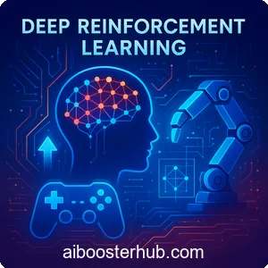
Deep Reinforcement Learning: Methods and Applications
Deep reinforcement learning (DRL) represents one of the most exciting frontiers in artificial intelligence, combining the decision-making power of reinforcement learning with the representation learning capabilities of deep neural networks. This powerful synthesis has enabled machines to master complex tasks ranging from playing Go at superhuman levels to controlling robotic systems with unprecedented precision. In this comprehensive guide, we’ll explore the foundations, methods, and real-world applications of deep reinforcement learning.
Content
Toggle1. Understanding deep reinforcement learning fundamentals
Deep reinforcement learning builds upon classical reinforcement learning by incorporating deep neural networks as function approximators. At its core, reinforcement learning in machine learning involves an agent that learns to make decisions by interacting with an environment. The agent receives observations, takes actions, and receives rewards that signal how well it’s performing.
The fundamental components of any DRL system include:
The agent represents the learner or decision-maker that observes the environment and selects actions. Unlike supervised learning where correct answers are provided, the agent must discover which actions yield the highest rewards through trial and error.
The environment encompasses everything the agent interacts with. It responds to the agent’s actions by transitioning to new states and providing reward signals. The environment can be fully or partially observable, deterministic or stochastic.
The state captures all relevant information about the current situation. In deep reinforcement learning, states are often high-dimensional, such as raw pixel values from images or complex sensor readings from robots.
Actions represent the choices available to the agent. These can be discrete (like choosing between specific moves in a game) or continuous (like adjusting the torque applied to a robot joint).
Rewards provide feedback about action quality. The reward function defines the agent’s objective, and the goal is to maximize cumulative reward over time.
The mathematical framework underlying reinforcement learning is the Markov Decision Process (MDP). An MDP is defined by a tuple \((S, A, P, R, \gamma)\) where \(S\) is the state space, \(A\) is the action space, \(P\) is the state transition probability, \(R\) is the reward function, and \(\gamma\) is the discount factor.
The agent’s goal is to learn a policy \(\pi(a|s)\) that maps states to actions in a way that maximizes the expected return:
$$ G_t = \sum_{k=0}^{\infty} \gamma^k R_{t+k+1} $$
Deep neural networks serve as powerful function approximators that can represent complex policies and value functions. This is where “deep” enters deep reinforcement learning – instead of using simple tabular methods or linear function approximation, we leverage multi-layer neural networks capable of learning hierarchical representations from raw sensory inputs.
2. Core reinforcement learning algorithms
The landscape of reinforcement learning algorithms can be broadly categorized into value-based methods, policy-based methods, and hybrid approaches that combine both. Understanding these categories is essential for selecting the right algorithm for your application.
Value-based methods
Value-based algorithms learn to estimate the value of being in a particular state or taking a particular action. The most influential value-based algorithm is Deep Q-Network (DQN), which revolutionized the field by successfully learning to play Atari games from raw pixels.
DQN learns an action-value function \(Q(s, a)\) that estimates the expected return for taking action \(a\) in state \(s\). The optimal action in any state is simply:
$$ a^* = \arg\max_a Q(s, a) $$
The Q-function is updated using the Bellman equation:
$$ Q(s, a) = R(s, a) + \gamma \max_{a’} Q(s’, a’) $$
In practice, DQN employs several key innovations including experience replay (storing and sampling past experiences) and target networks (using a separate, slowly-updated network for computing targets). Here’s a simplified implementation of the core DQN update:
import numpy as np
import torch
import torch.nn as nn
import torch.optim as optim

class DQN(nn.Module):
    def __init__(self, state_dim, action_dim):
        super(DQN, self).__init__()
        self.fc1 = nn.Linear(state_dim, 128)
        self.fc2 = nn.Linear(128, 128)
        self.fc3 = nn.Linear(128, action_dim)

    def forward(self, x):
        x = torch.relu(self.fc1(x))
        x = torch.relu(self.fc2(x))
        return self.fc3(x)

# Training step
def update_dqn(q_network, target_network, optimizer, batch, gamma=0.99):
    states, actions, rewards, next_states, dones = batch

    # Current Q values
    current_q = q_network(states).gather(1, actions.unsqueeze(1))

    # Target Q values
    with torch.no_grad():
        next_q = target_network(next_states).max(1)[0]
        target_q = rewards + gamma * next_q * (1 - dones)

    # Compute loss and update
    loss = nn.MSELoss()(current_q.squeeze(), target_q)
    optimizer.zero_grad()
    loss.backward()
    optimizer.step()

    return loss.item()
Policy gradient methods
While value-based methods learn which actions are best indirectly through value estimation, policy gradient methods directly optimize the policy itself. This approach is particularly powerful for problems with continuous action spaces or stochastic optimal policies.
The policy gradient theorem provides the foundation for these methods. It states that the gradient of the expected return with respect to policy parameters \(\theta\) is:
$$\nabla_\theta J(\theta) =
\mathbb{E}_{\pi_\theta} \left[
\nabla_\theta \log \pi_\theta(a \mid s) \, Q^{\pi}(s, a)
\right]$$
REINFORCE, one of the simplest policy gradient algorithms, uses Monte Carlo samples to estimate this gradient:
class PolicyNetwork(nn.Module):
    def __init__(self, state_dim, action_dim):
        super(PolicyNetwork, self).__init__()
        self.fc1 = nn.Linear(state_dim, 128)
        self.fc2 = nn.Linear(128, action_dim)

    def forward(self, x):
        x = torch.relu(self.fc1(x))
        return torch.softmax(self.fc2(x), dim=-1)

def reinforce_update(policy, optimizer, episode_data, gamma=0.99):
    states, actions, rewards = episode_data

    # Calculate discounted returns
    returns = []
    G = 0
    for r in reversed(rewards):
        G = r + gamma * G
        returns.insert(0, G)
    returns = torch.tensor(returns)

    # Normalize returns
    returns = (returns - returns.mean()) / (returns.std() + 1e-8)

    # Calculate policy loss
    loss = 0
    for state, action, G in zip(states, actions, returns):
        probs = policy(state)
        log_prob = torch.log(probs[action])
        loss += -log_prob * G

    # Update policy
    optimizer.zero_grad()
    loss.backward()
    optimizer.step()
Actor-critic architectures
Actor-critic methods combine the best of both worlds by maintaining both a policy (the actor) and a value function (the critic). The actor decides which actions to take, while the critic evaluates those actions, providing lower-variance gradient estimates than pure policy gradient methods.
The advantage function \(A(s, a) = Q(s, a) – V(s)\) plays a central role in actor-critic algorithms. It measures how much better an action is compared to the average action in that state. This reduces variance in policy gradient estimates while maintaining unbiased gradient directions.
Advantage Actor-Critic (A2C) is a popular synchronous variant that updates both actor and critic networks:
class ActorCritic(nn.Module):
    def __init__(self, state_dim, action_dim):
        super(ActorCritic, self).__init__()
        self.shared = nn.Linear(state_dim, 128)
        self.actor = nn.Linear(128, action_dim)
        self.critic = nn.Linear(128, 1)

    def forward(self, x):
        x = torch.relu(self.shared(x))
        action_probs = torch.softmax(self.actor(x), dim=-1)
        state_value = self.critic(x)
        return action_probs, state_value

def a2c_update(model, optimizer, states, actions, rewards, next_states, dones, gamma=0.99):
    # Forward pass
    action_probs, values = model(states)
    _, next_values = model(next_states)

    # Calculate TD error (advantage)
    td_target = rewards + gamma * next_values * (1 - dones)
    advantages = td_target - values

    # Actor loss (policy gradient)
    log_probs = torch.log(action_probs.gather(1, actions.unsqueeze(1)))
    actor_loss = -(log_probs * advantages.detach()).mean()

    # Critic loss (value function)
    critic_loss = advantages.pow(2).mean()

    # Combined loss
    loss = actor_loss + 0.5 * critic_loss

    optimizer.zero_grad()
    loss.backward()
    optimizer.step()
3. Continuous control with deep reinforcement learning
While many early successes in DRL focused on discrete action spaces like game-playing, continuous control problems present unique challenges and opportunities. Tasks like robotic manipulation, autonomous driving, and continuous resource allocation require algorithms that can handle infinite action spaces.
The challenge of continuous actions
In continuous control, the action space is typically represented as a vector of real numbers, often bounded within specific ranges. For example, controlling a robotic arm might require specifying continuous joint angles or torques. The dimensionality of these action spaces can be quite high – a humanoid robot might have dozens of controllable joints.
Traditional value-based methods like DQN struggle here because finding (\max_a Q(s, a)) requires solving an optimization problem at every step. While theoretically possible, this is computationally expensive and can be unstable.
Deep Deterministic Policy Gradient (DDPG)
Deep Deterministic Policy Gradient (DDPG) was specifically designed for continuous control with deep reinforcement learning. DDPG is an actor-critic algorithm that learns a deterministic policy, meaning it outputs a specific action rather than a probability distribution over actions.
The key innovation in DDPG is treating the Q-function as a differentiable function of actions. This allows us to compute the policy gradient directly:
$$\nabla_\theta J \approx
\mathbb{E}_{s \sim \rho} \left[
\nabla_a Q(s, a) \big|_{a = \mu_\theta(s)} \,
\nabla_\theta \mu_\theta(s)
\right]$$
Here’s a simplified implementation of the DDPG algorithm:
class Actor(nn.Module):
    def __init__(self, state_dim, action_dim, max_action):
        super(Actor, self).__init__()
        self.fc1 = nn.Linear(state_dim, 256)
        self.fc2 = nn.Linear(256, 256)
        self.fc3 = nn.Linear(256, action_dim)
        self.max_action = max_action

    def forward(self, state):
        x = torch.relu(self.fc1(state))
        x = torch.relu(self.fc2(x))
        x = torch.tanh(self.fc3(x))
        return x * self.max_action

class Critic(nn.Module):
    def __init__(self, state_dim, action_dim):
        super(Critic, self).__init__()
        self.fc1 = nn.Linear(state_dim + action_dim, 256)
        self.fc2 = nn.Linear(256, 256)
        self.fc3 = nn.Linear(256, 1)

    def forward(self, state, action):
        x = torch.cat([state, action], dim=1)
        x = torch.relu(self.fc1(x))
        x = torch.relu(self.fc2(x))
        return self.fc3(x)

def ddpg_update(actor, critic, target_actor, target_critic,
                actor_optimizer, critic_optimizer, batch, gamma=0.99):
    states, actions, rewards, next_states, dones = batch

    # Update critic
    with torch.no_grad():
        next_actions = target_actor(next_states)
        target_q = rewards + gamma * target_critic(next_states, next_actions) * (1 - dones)

    current_q = critic(states, actions)
    critic_loss = nn.MSELoss()(current_q, target_q)

    critic_optimizer.zero_grad()
    critic_loss.backward()
    critic_optimizer.step()

    # Update actor
    actor_loss = -critic(states, actor(states)).mean()

    actor_optimizer.zero_grad()
    actor_loss.backward()
    actor_optimizer.step()

    # Soft update target networks
    tau = 0.005
    for param, target_param in zip(critic.parameters(), target_critic.parameters()):
        target_param.data.copy_(tau * param.data + (1 - tau) * target_param.data)

    for param, target_param in zip(actor.parameters(), target_actor.parameters()):
        target_param.data.copy_(tau * param.data + (1 - tau) * target_param.data)
DDPG incorporates several important techniques including target networks (both for actor and critic), experience replay for breaking temporal correlations, and exploration noise added to actions during training. The Ornstein-Uhlenbeck process is commonly used to generate temporally correlated exploration noise:
class OUNoise:
    def __init__(self, action_dim, mu=0, theta=0.15, sigma=0.2):
        self.action_dim = action_dim
        self.mu = mu
        self.theta = theta
        self.sigma = sigma
        self.state = np.ones(self.action_dim) * self.mu

    def reset(self):
        self.state = np.ones(self.action_dim) * self.mu

    def sample(self):
        dx = self.theta * (self.mu - self.state) + self.sigma * np.random.randn(self.action_dim)
        self.state += dx
        return self.state
Twin Delayed DDPG (TD3)
Building on DDPG, Twin Delayed DDPG (TD3) addresses several issues including overestimation bias in value functions. TD3 uses three key tricks: using two Q-functions and taking the minimum to reduce overestimation, delaying policy updates relative to value updates, and adding noise to target actions for smoothing.
Soft Actor-Critic (SAC)
Another powerful approach for continuous control is Soft Actor-Critic (SAC), which incorporates entropy regularization to encourage exploration. SAC learns a stochastic policy that maximizes both expected return and entropy:
$$ J(\pi) = \sum_t \mathbb{E}\left[r(s_t, a_t) + \alpha \mathcal{H}(\pi(\cdot|s_t))\right] $$
where \(\mathcal{H}\) is the entropy function and \(\alpha\) controls the trade-off between exploitation and exploration. SAC has demonstrated remarkable sample efficiency and robustness across various continuous control tasks.
4. Deep reinforcement learning from human preferences
One of the most significant challenges in applying DRL to real-world problems is reward specification. Designing reward functions that accurately capture desired behavior is often difficult or even impossible for complex tasks. Deep reinforcement learning from human preferences (RLHF) offers an elegant solution by learning reward functions from human feedback.
The reward specification problem
Consider teaching an AI to write helpful responses. How would you define a reward function? You might try measuring response length, keyword matches, or grammatical correctness, but these proxies often miss the essence of what makes a response truly helpful. The agent might exploit these metrics in unexpected ways – writing verbose but unhelpful responses, or grammatically perfect but irrelevant text.
This challenge becomes even more pronounced in domains like robotics, where we want agents to perform tasks “naturally” or “safely” – qualities that are easy for humans to judge but hard to formalize mathematically.
Learning from comparisons
The core insight of RLHF is that humans are much better at comparing outcomes than assigning absolute scores. Given two robot trajectories, you can easily say which one looks more natural. Given two text responses, you can identify which is more helpful. This comparative feedback is more reliable, consistent, and easier to provide than numerical rewards.
The RLHF process typically involves three stages:
Demonstration collection: First, collect a dataset of behavior through human demonstrations, random exploration, or a preliminary policy. This provides diverse examples of the task.
Reward learning: Present pairs of trajectories to human evaluators who indicate their preference. Train a reward model to predict these preferences using a binary classification objective:
$$\mathcal{L}(\theta) =
– \mathbb{E}_{(\sigma^1, \sigma^2, \mu) \sim D} \left[
\mu \, \log \hat{P}_\theta(\sigma^1 \succ \sigma^2)
+ (1 – \mu) \, \log \hat{P}_\theta(\sigma^2 \succ \sigma^1)
\right]$$
where \(\sigma^1\) and \(\sigma^2\) are trajectory segments, \(\mu \in {0,1}\) indicates which is preferred, and \(\hat{P}_\theta\) is the preference prediction from the reward model.
Policy optimization: Use the learned reward model as the reward function for standard RL algorithms. The agent now optimizes for human preferences rather than a hand-designed reward.
Here’s a conceptual implementation of reward model training:
class RewardModel(nn.Module):
    def __init__(self, state_dim, action_dim):
        super(RewardModel, self).__init__()
        self.fc1 = nn.Linear(state_dim + action_dim, 256)
        self.fc2 = nn.Linear(256, 256)
        self.fc3 = nn.Linear(256, 1)

    def forward(self, states, actions):
        x = torch.cat([states, actions], dim=-1)
        x = torch.relu(self.fc1(x))
        x = torch.relu(self.fc2(x))
        return self.fc3(x)

    def get_trajectory_reward(self, trajectory):
        states, actions = trajectory
        rewards = self.forward(states, actions)
        return rewards.sum()

def train_reward_model(model, optimizer, comparison_data):
    """
    comparison_data: list of (trajectory_1, trajectory_2, preference)
    where preference is 0 if trajectory_1 is preferred, 1 if trajectory_2 is preferred
    """
    losses = []

    for traj1, traj2, preference in comparison_data:
        # Get predicted rewards for both trajectories
        reward1 = model.get_trajectory_reward(traj1)
        reward2 = model.get_trajectory_reward(traj2)

        # Compute preference probability using Bradley-Terry model
        logits = reward1 - reward2
        predicted_pref = torch.sigmoid(logits)

        # Cross-entropy loss
        target = torch.tensor([1.0 - preference], dtype=torch.float32)
        loss = nn.BCELoss()(predicted_pref, target)

        optimizer.zero_grad()
        loss.backward()
        optimizer.step()

        losses.append(loss.item())

    return np.mean(losses)
Applications and impact
RLHF has become instrumental in training large language models, enabling systems to align with human values and preferences without explicit reward engineering. Beyond language models, RLHF has been successfully applied to robotic manipulation (learning natural grasping behaviors), autonomous vehicles (learning comfortable driving styles), and game AI (learning to play games in human-like ways).
The iterative nature of RLHF is particularly powerful. As policies improve, you can collect new trajectories that explore previously unseen regions of the state space, then gather preferences on these new behaviors to refine the reward model. This creates a virtuous cycle of continuous improvement.
5. Advanced topics in DRL
As deep reinforcement learning continues to evolve, several advanced techniques have emerged to address specific challenges and push the boundaries of what’s possible.
Multi-agent reinforcement learning
Real-world systems often involve multiple agents that must coordinate or compete. Multi-agent reinforcement learning (MARL) extends DRL to these settings. The key challenge is non-stationarity: from any agent’s perspective, the environment is constantly changing because other agents are simultaneously learning and adapting.
Approaches to MARL include independent learning (each agent learns independently), centralized training with decentralized execution (agents share information during training but act independently at test time), and communication protocols (agents learn to share information explicitly).
Model-based reinforcement learning
While most DRL algorithms are model-free (they don’t explicitly learn environment dynamics), model-based RL learns a predictive model of how the environment responds to actions. This model can be used for planning, generating synthetic training data, or providing auxiliary learning signals.
The core idea is learning a dynamics model \(s_{t+1} = f(s_t, a_t)\) and using it to simulate trajectories:
class WorldModel(nn.Module):
    def __init__(self, state_dim, action_dim):
        super(WorldModel, self).__init__()
        self.fc1 = nn.Linear(state_dim + action_dim, 256)
        self.fc2 = nn.Linear(256, 256)
        self.fc3 = nn.Linear(256, state_dim)

    def forward(self, state, action):
        x = torch.cat([state, action], dim=-1)
        x = torch.relu(self.fc1(x))
        x = torch.relu(self.fc2(x))
        return self.fc3(x)

    def predict_trajectory(self, initial_state, actions):
        states = [initial_state]
        current_state = initial_state

        for action in actions:
            next_state = self.forward(current_state, action)
            states.append(next_state)
            current_state = next_state

        return torch.stack(states)
Model-based approaches can be significantly more sample-efficient than model-free methods, but they face challenges with model errors compounding over long horizons.
Offline reinforcement learning
Traditional RL assumes the agent can interact with the environment to collect new data. Offline RL (also called batch RL) learns from fixed datasets without additional interaction. This is crucial for domains where data collection is expensive, dangerous, or impossible.
The main challenge is distribution shift: the learned policy may select actions not well-represented in the dataset, leading to unreliable value estimates. Conservative Q-Learning (CQL) addresses this by penalizing Q-values for out-of-distribution actions:
$$\min_{Q} \;
\alpha \, \mathbb{E}_{s \sim D, \; a \sim \mu(a \mid s)} \big[ Q(s, a) \big]
+ \mathbb{E}_{s, a, r, s’ \sim D} \big[ \big( Q(s, a) – \mathcal{B}^\pi Q(s, a) \big)^2 \big] $$
Hierarchical reinforcement learning
Complex tasks often have natural hierarchical structure – to make breakfast, you must first prepare ingredients, then cook them, then serve them. Hierarchical RL learns policies at multiple levels of abstraction, with high-level policies selecting goals or sub-tasks and low-level policies executing them.
Options framework and feudal reinforcement learning are popular approaches that enable agents to learn reusable skills and long-horizon planning.
6. Real-world applications and case studies
Deep reinforcement learning has transcended academic research to deliver practical impact across numerous domains. Understanding these applications provides insight into both the potential and current limitations of DRL.
Game playing and simulated environments
DRL first captured widespread attention through remarkable achievements in games. AlphaGo’s victory over world champion Go players demonstrated that DRL could master tasks requiring intuition and long-term planning. The algorithm combined Monte Carlo tree search with deep neural networks trained through self-play.
Modern game-playing agents have extended far beyond board games. OpenAI Five mastered Dota 2, a complex multiplayer video game with imperfect information and enormous action spaces. AlphaStar achieved grandmaster level in StarCraft II, handling real-time strategy, resource management, and adversarial planning simultaneously.
These successes aren’t merely about games – they represent testbeds for developing algorithms that handle complexity, uncertainty, and strategic reasoning applicable to real-world problems.
Robotics and control systems
Robotics represents one of the most promising application areas for DRL. Learning dexterous manipulation – teaching robots to handle objects with human-like finesse – has seen tremendous progress through algorithms like DDPG and SAC.
Industrial robots now learn optimal control policies for tasks like assembly, welding, and packaging. Rather than programming every movement explicitly, engineers can define objectives and let DRL discover efficient solutions. This is particularly valuable when dealing with variations in materials, lighting conditions, or object positions.
Legged locomotion is another success story. Robots trained with DRL have learned to walk, run, and navigate rough terrain more robustly than traditionally programmed systems. The key is that RL can discover adaptive behaviors that respond dynamically to perturbations and unexpected situations.
Autonomous vehicles
Self-driving cars employ DRL for various sub-tasks including path planning, decision-making at intersections, and adapting to driver preferences. While end-to-end learning (directly from sensors to controls) remains challenging for safety-critical deployment, DRL excels at learning specific maneuvers in simulation before validation on real vehicles.
Adaptive cruise control, lane-keeping assistance, and parking automation have all benefited from reinforcement learning approaches. These systems learn to balance multiple objectives: safety, efficiency, passenger comfort, and traffic flow.
Resource management and optimization
DRL has proven remarkably effective for resource allocation problems. Data center cooling, where Google applied DRL to reduce energy consumption by significant percentages, demonstrates the practical value. The agent learns to predict thermal dynamics and optimize cooling strategies continuously.
In cloud computing, DRL manages workload distribution across servers, balancing performance, energy efficiency, and hardware wear. Financial trading systems use reinforcement learning for portfolio management, learning to adapt strategies to changing market conditions.
Energy grid management increasingly relies on DRL to balance supply and demand, integrate renewable sources, and optimize storage deployment. These applications showcase DRL’s ability to handle complex, continuous optimization problems in dynamic environments.
Healthcare and personalized treatment
Medical treatment planning is inherently sequential – decisions at each stage affect future options and outcomes. DRL shows promise in optimizing chemotherapy schedules, ventilator settings for critically ill patients, and personalized medication dosages.
Sepsis treatment, where clinicians must make rapid decisions about fluid administration and vasopressor use, has been studied extensively using offline RL on historical patient data. While clinical deployment requires rigorous validation, these systems can suggest treatment strategies and highlight potential risks.
Natural language and content recommendation
Large language models increasingly use reinforcement learning from human preferences to align outputs with user intent. Rather than simply predicting the next word, these models learn to generate helpful, harmless, and honest responses based on human feedback.
Content recommendation systems on streaming platforms, e-commerce sites, and social media employ multi-armed bandit algorithms and contextual bandits (simplified RL settings) to personalize suggestions. These systems balance exploration of new content with exploitation of known user preferences, continuously learning from user interactions.
7. Conclusion
Deep reinforcement learning represents a paradigm shift in how we approach sequential decision-making problems. By combining the representation power of deep neural networks with the adaptive learning framework of reinforcement learning, DRL has enabled machines to master tasks once thought to require human-level intelligence. From continuous control with deep reinforcement learning in robotics to deep reinforcement learning from human preferences in language models, the field continues to expand its reach and impact.
The journey from understanding basic reinforcement learning algorithms like policy gradient and actor-critic methods to implementing sophisticated techniques like DDPG and RLHF illustrates both the elegance and complexity of this field. While challenges remain – including sample efficiency, safety assurance, and reward specification – the rapid progress and diverse applications of DRL suggest a future where intelligent systems can learn and adapt to increasingly complex real-world scenarios. As practitioners and researchers continue to refine these methods, deep reinforcement learning will undoubtedly play a central role in shaping the next generation of AI systems.
8. Knowledge Check
Quiz 1: Fundamentals of Deep Reinforcement Learning
Question: Describe the five fundamental components of a Deep Reinforcement Learning (DRL) system as outlined in the text.
Answer: A DRL system consists of five essential components. First, the agent serves as the learner or decision-maker. It discovers optimal actions through trial and error. Second, the environment encompasses everything the agent interacts with.
Quiz 2: Value-Based Learning Methods
Question: What is the primary function of the Deep Q-Network (DQN) algorithm, and what two key innovations does it employ to stabilize learning?
Answer: DQN became famous for learning Atari games from raw pixels. Its primary function is learning an action-value function, Q(s, a). This function estimates the expected return for specific actions in given states.
Quiz 3: Policy Gradient Methods
Question: How do policy gradient methods differ from value-based methods, and for what types of problems are they particularly powerful?
Answer: Policy gradient methods differ fundamentally from value-based approaches. Unlike value-based methods, they directly optimize the policy itself. In contrast, value-based methods learn action values first, then derive policies.
Quiz 4: Actor-Critic Architectures
Question: Explain the roles of the ‘actor’ and the ‘critic’ in an actor-critic architecture and define the advantage function.
Answer: Actor-critic architectures combine two essential components. The actor represents the policy that selects actions. Meanwhile, the critic is a value function that evaluates those actions.
Quiz 5: Continuous Control Algorithms
Question: Why do traditional value-based methods like DQN struggle with continuous action spaces, and how does Deep Deterministic Policy Gradient (DDPG) overcome this challenge?
Answer: DQN faces challenges with continuous action spaces. Finding the action that maximizes Q-value requires optimization at every step. This becomes computationally expensive.
Quiz 6: Learning from Human Preferences
Question: What is the core problem that Reinforcement Learning from Human Preferences (RLHF) is designed to solve, and what is the three-stage process it typically follows?
Answer: RLHF addresses the reward specification problem. Defining reward functions is often difficult. Instead, it leverages human comparison abilities. Humans excel at comparing outcomes rather than assigning absolute scores.
The process follows three stages:
- Demonstration collection gathers diverse examples
- Reward learning trains a model to predict human preferences between outcome pairs
- Policy optimization uses the learned reward model to improve the agent’s policy
Therefore, this approach enables more natural reward specification.
Quiz 7: Advanced DRL: Model-Based vs. Model-Free
Question: What is the key difference between model-free and model-based reinforcement learning, and what is the main advantage of the model-based approach?
Answer: The key difference lies in their learning approach. Model-free RL learns policies or value functions directly from experience. In contrast, model-based RL first learns a predictive model of environment dynamics.
Quiz 8: Advanced DRL: Offline Learning
Question: Define Offline Reinforcement Learning and explain the main challenge it faces, known as distribution shift.
Answer: Offline RL (also called batch RL) learns from fixed datasets. It requires no further environment interaction. This makes it valuable for real-world applications.
Quiz 9: Applications in Gaming and Robotics
Question: Name two games mentioned in the text where DRL agents achieved superhuman or grandmaster-level performance, and describe a key application of DRL in robotics.
Answer: DRL achieved remarkable success in competitive gaming. AlphaGo mastered the game of Go with superhuman performance. Similarly, AlphaStar reached grandmaster level in StarCraft II.
Quiz 10: Applications in Resource Management and NLP
Question: Describe how DRL has been applied for resource management in data centers and how it is used to align large language models.
Answer: DRL transformed data center efficiency. Google used it to reduce energy consumption significantly. The system learns to predict thermal dynamics. Then, it optimizes cooling strategies accordingly.

