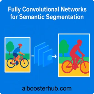
Fully Convolutional Networks for Semantic Segmentation
Semantic segmentation represents one of the most challenging tasks in computer vision, requiring pixel-level understanding of images. Unlike traditional image classification that assigns a single label to an entire image, semantic segmentation assigns a class label to every pixel, effectively creating a detailed map of what appears where in an image. Fully convolutional networks (FCN) revolutionized this field by adapting powerful classification architectures for dense prediction tasks, enabling end-to-end learning without the need for hand-crafted features or complex post-processing.
The breakthrough of fully convolutional networks for semantic segmentation lies in their elegant architecture that replaces fully connected layers with convolutional layers, allowing networks to accept images of any size and produce correspondingly-sized output maps. This architectural innovation, combined with techniques like skip connections and upsampling, has become the foundation for modern semantic segmentation systems and has inspired numerous variants, including the widely-used U-Net convolutional networks for biomedical image segmentation.
1. Understanding semantic segmentation and its challenges
Semantic segmentation requires assigning a class label to each pixel in an image, creating a dense prediction across the entire spatial domain. This task differs fundamentally from image classification, which outputs a single label, and object detection, which predicts bounding boxes around objects. In semantic segmentation, we need to understand not just what objects are present, but precisely where they are located at the pixel level.
What makes semantic segmentation difficult
The primary challenge in semantic segmentation is maintaining spatial resolution while capturing semantic information. Traditional convolutional neural networks designed for classification progressively reduce spatial dimensions through pooling and striding, creating feature maps that are excellent for understanding what is in an image but poor for understanding where things are located. This presents a fundamental trade-off: we need large receptive fields to capture context, but we also need fine spatial resolution to make accurate pixel-level predictions.
Another significant challenge is class imbalance. In many real-world scenarios, certain classes dominate the image while others occupy only small regions. For example, in street scene segmentation, the “road” class might cover 60% of pixels while a “traffic sign” class covers less than 1%. This imbalance makes training difficult, as the network can achieve high accuracy by simply predicting the dominant class everywhere.
Applications across domains
Semantic segmentation has found applications in numerous domains. In autonomous driving, it enables vehicles to understand their surroundings by segmenting roads, pedestrians, vehicles, and other objects. Medical imaging relies heavily on semantic segmentation for tasks like tumor detection, organ segmentation, and tissue classification. Satellite imagery analysis uses semantic segmentation for land cover classification, urban planning, and environmental monitoring. These diverse applications demonstrate why developing robust semantic segmentation systems is crucial for AI progress.
2. The architecture of fully convolutional networks
The key innovation of fully convolutional networks lies in their architecture, which eliminates fully connected layers entirely. Traditional CNNs for classification consist of convolutional layers followed by fully connected layers that flatten the spatial dimensions and produce a fixed-size output vector. This architecture is incompatible with dense prediction tasks because it discards spatial information and requires fixed-size inputs.
Converting classification networks to fully convolutional
Fully convolutional networks transform classification architectures by replacing fully connected layers with convolutional layers. Consider a typical classification network like VGG-16, which might have fully connected layers with 4096 neurons. We can replace these with 1×1 convolutional layers that preserve spatial structure. If the input to the first fully connected layer would have been 7×7×512, we can instead use a 1×1 convolution with 4096 filters, producing a 7×7×4096 output that maintains spatial organization.
This transformation has profound implications. The resulting network can now accept inputs of any size, not just the fixed size it was trained on. More importantly, the output is not a single vector but a spatial map, with each location in the output corresponding to a receptive field in the input. This spatial correspondence is exactly what we need for semantic segmentation.
The encoder-decoder structure
FCN architectures typically follow an encoder-decoder pattern. The encoder portion consists of the convolutional and pooling layers from the original classification network, progressively reducing spatial dimensions while increasing the number of channels. This creates a compressed representation that captures semantic information but with reduced spatial resolution.
The decoder portion upsamples these coarse feature maps back to the original image resolution. The simplest approach uses bilinear upsampling or transposed convolutions (also called deconvolutions). A transposed convolution can be thought of as performing convolution in the opposite direction, expanding spatial dimensions rather than reducing them. For upsampling by a factor of 2, we might use a transposed convolution with a 4×4 kernel and stride 2.
Here’s a simple implementation of the upsampling portion:
import torch
import torch.nn as nn

class FCNDecoder(nn.Module):
    def __init__(self, in_channels, num_classes):
        super(FCNDecoder, self).__init__()

        # Transposed convolution for 2x upsampling
        self.upsample_2x = nn.ConvTranspose2d(
            in_channels,
            in_channels // 2,
            kernel_size=4,
            stride=2,
            padding=1
        )

        # Transposed convolution for 4x upsampling
        self.upsample_4x = nn.ConvTranspose2d(
            in_channels // 2,
            in_channels // 4,
            kernel_size=4,
            stride=2,
            padding=1
        )

        # Final upsampling to original resolution
        self.upsample_8x = nn.ConvTranspose2d(
            in_channels // 4,
            num_classes,
            kernel_size=16,
            stride=8,
            padding=4
        )

    def forward(self, x):
        x = torch.relu(self.upsample_2x(x))
        x = torch.relu(self.upsample_4x(x))
        x = self.upsample_8x(x)
        return x
3. Skip connections and multi-scale fusion
One of the most important innovations in fully convolutional networks is the use of skip connections to combine information from multiple scales. While the encoder-decoder structure can upsample coarse predictions back to full resolution, this approach alone produces predictions with blurry boundaries and missed fine details. Skip connections address this limitation by fusing features from different levels of the network.
Why skip connections matter
As information flows through the encoder, early layers capture fine-grained details like edges and textures, while deeper layers capture high-level semantic information. When we upsample only from the deepest layer, we’re trying to recover fine spatial details from a highly compressed representation that has lost much of that information. Skip connections allow the decoder to access features from earlier layers that still contain fine spatial details.
The original FCN paper introduced three variants: FCN-32s, FCN-16s, and FCN-8s. FCN-32s upsamples predictions directly from the final layer by a factor of 32. FCN-16s adds a skip connection from an earlier layer, combining it with 2× upsampled predictions before final upsampling. FCN-8s adds another skip connection, creating even more refined predictions. Each additional skip connection improved segmentation accuracy, particularly around object boundaries.
Implementing skip connections
Skip connections require careful handling of spatial dimensions and channel numbers. Features from different layers have different spatial resolutions and channel counts, so we need to align them before combining. Typically, this involves upsampling the deeper features and optionally using 1×1 convolutions to match channel dimensions.
Here’s an implementation showing how to combine features from multiple scales:
class FCNWithSkips(nn.Module):
    def __init__(self, num_classes):
        super(FCNWithSkips, self).__init__()

        # Assuming we have encoder features at different scales
        # pool3: 1/8 resolution, 256 channels
        # pool4: 1/16 resolution, 512 channels
        # pool5: 1/32 resolution, 512 channels

        # 1x1 conv to reduce channels from pool4
        self.score_pool4 = nn.Conv2d(512, num_classes, 1)

        # 1x1 conv to reduce channels from pool3
        self.score_pool3 = nn.Conv2d(256, num_classes, 1)

        # 1x1 conv for final prediction
        self.score_pool5 = nn.Conv2d(512, num_classes, 1)

        # Upsampling layers
        self.upsample_2x = nn.ConvTranspose2d(
            num_classes, num_classes,
            kernel_size=4, stride=2, padding=1
        )

        self.upsample_8x = nn.ConvTranspose2d(
            num_classes, num_classes,
            kernel_size=16, stride=8, padding=4
        )

    def forward(self, pool3, pool4, pool5):
        # Score pool5 and upsample 2x
        score_pool5 = self.score_pool5(pool5)
        upsample_pool5 = self.upsample_2x(score_pool5)

        # Score pool4 and add
        score_pool4 = self.score_pool4(pool4)
        fused_pool4 = upsample_pool5 + score_pool4

        # Upsample fused result 2x
        upsample_pool4 = self.upsample_2x(fused_pool4)

        # Score pool3 and add
        score_pool3 = self.score_pool3(pool3)
        fused_pool3 = upsample_pool4 + score_pool3

        # Final 8x upsampling to original resolution
        output = self.upsample_8x(fused_pool3)

        return output
The mathematics of feature fusion
When combining features from different scales, we’re essentially performing a weighted sum of predictions at different resolutions. Let ( F_i ) represent features at scale ( i ), and ( U ) represent an upsampling operation. The fused prediction ( P ) can be expressed as:
$$ P = U^{32}(F_5) + U^{16}(F_4) + U^8(F_3) $$
Where \( U^n \) denotes upsampling by a factor of \( n \). In practice, this fusion is performed progressively rather than all at once, allowing the network to learn optimal weights for combining different scales during training.
4. Training fully convolutional networks
Training fully convolutional networks for semantic segmentation involves several considerations beyond standard classification training. The loss function, data augmentation strategies, and training procedures all need to be adapted for dense prediction tasks.
Loss functions for semantic segmentation
The most common loss function for semantic segmentation is pixel-wise cross-entropy. For each pixel, we compute the cross-entropy between the predicted class distribution and the ground truth label. The total loss is the average across all pixels. Mathematically, for an image with \( N \) pixels and \( C \) classes, the loss is:
$$ L = -\frac{1}{N} \sum_{i=1}^{N} \sum_{c=1}^{C} y_{i,c} \log(p_{i,c}) $$
Where \( y_{i,c} \) is 1 if pixel \( i \) belongs to class \( c \) and 0 otherwise, and \( p_{i,c} \) is the predicted probability that pixel \( i \) belongs to class \( c \).
However, standard cross-entropy doesn’t address class imbalance. Several modifications have been proposed, including weighted cross-entropy that assigns higher weights to rare classes, and focal loss that focuses learning on hard examples. The focal loss adds a modulating factor to down-weight easy examples:
$$ L_{focal} = -\frac{1}{N} \sum_{i=1}^{N} \sum_{c=1}^{C} (1 – p_{i,c})^\gamma y_{i,c} \log(p_{i,c}) $$
Where \( \gamma \) is a focusing parameter, typically set to 2.
Implementation of training loop
Here’s a practical implementation of training a FCN model:
import torch
import torch.nn as nn
import torch.optim as optim
from torch.utils.data import DataLoader

def train_fcn(model, train_loader, num_epochs, device='cuda'):
    """
    Train a fully convolutional network for semantic segmentation
    """
    model = model.to(device)
    criterion = nn.CrossEntropyLoss()
    optimizer = optim.Adam(model.parameters(), lr=1e-4)

    # Learning rate scheduler
    scheduler = optim.lr_scheduler.ReduceLROnPlateau(
        optimizer, mode='min', factor=0.5, patience=5
    )

    for epoch in range(num_epochs):
        model.train()
        total_loss = 0

        for batch_idx, (images, masks) in enumerate(train_loader):
            images = images.to(device)
            masks = masks.to(device)

            # Forward pass
            outputs = model(images)

            # Compute loss
            loss = criterion(outputs, masks)

            # Backward pass and optimization
            optimizer.zero_grad()
            loss.backward()
            optimizer.step()

            total_loss += loss.item()

            if batch_idx % 100 == 0:
                print(f'Epoch [{epoch+1}/{num_epochs}], '
                      f'Step [{batch_idx}/{len(train_loader)}], '
                      f'Loss: {loss.item():.4f}')

        avg_loss = total_loss / len(train_loader)
        scheduler.step(avg_loss)
        print(f'Epoch [{epoch+1}/{num_epochs}], Average Loss: {avg_loss:.4f}')

def compute_iou(predictions, targets, num_classes):
    """
    Compute Intersection over Union (IoU) for each class
    """
    ious = []
    predictions = predictions.view(-1)
    targets = targets.view(-1)

    for cls in range(num_classes):
        pred_inds = predictions == cls
        target_inds = targets == cls
        intersection = (pred_inds & target_inds).sum().float()
        union = (pred_inds | target_inds).sum().float()

        if union == 0:
            ious.append(float('nan'))
        else:
            ious.append((intersection / union).item())

    return ious
Data augmentation strategies
Data augmentation is crucial for training robust segmentation models. Unlike classification where we can use aggressive transformations, semantic segmentation requires that augmentations preserve the correspondence between images and segmentation masks. Common augmentations include random scaling, random cropping, horizontal flipping, and color jittering. Both the image and mask must undergo identical geometric transformations.
5. U-Net: A specialized architecture for biomedical image segmentation
While the original fully convolutional networks demonstrated the power of end-to-end learning for semantic segmentation, U-Net convolutional networks for biomedical image segmentation introduced several architectural refinements that made them particularly effective for medical imaging tasks. The U-Net architecture has become one of the most influential designs in medical image analysis.
The U-Net architecture
U-Net follows a symmetric encoder-decoder structure that resembles the letter “U,” hence its name. The encoder (contracting path) follows the typical architecture of convolutional networks, with repeated application of convolutions followed by max pooling for downsampling. The decoder (expansive path) consists of upsampling followed by convolutions, gradually recovering spatial resolution.
The key distinguishing feature of U-Net is its extensive use of skip connections. Unlike FCN which adds skip connections from a few specific layers, U-Net connects every layer in the encoder to its corresponding layer in the decoder. These connections concatenate feature maps rather than adding them, allowing the decoder to access both high-level semantic information from the bottleneck and fine-grained spatial information from the encoder.
Why U-Net excels in medical imaging
U-Net convolutional networks for biomedical image segmentation address several challenges specific to medical imaging. First, medical imaging datasets are often small due to the cost and difficulty of obtaining labeled data. U-Net’s architecture with skip connections provides strong regularization, helping the network learn effectively from limited data. Second, medical images often require precise boundary localization, such as delineating tumor margins. The concatenated skip connections in U-Net preserve fine spatial details that enable accurate boundary detection.
The architecture also incorporates data augmentation strategies tailored for medical imaging. Random elastic deformations, which simulate tissue deformation, are particularly effective for training on small medical imaging datasets. This augmentation, combined with U-Net’s architecture, allows training with as few as 30 annotated images in some cases.
Implementing a U-Net architecture
Here’s a complete implementation of the U-Net architecture:
class UNet(nn.Module):
    def __init__(self, in_channels=3, num_classes=2):
        super(UNet, self).__init__()

        # Encoder (contracting path)
        self.enc1 = self.conv_block(in_channels, 64)
        self.enc2 = self.conv_block(64, 128)
        self.enc3 = self.conv_block(128, 256)
        self.enc4 = self.conv_block(256, 512)

        # Bottleneck
        self.bottleneck = self.conv_block(512, 1024)

        # Decoder (expansive path)
        self.upconv4 = nn.ConvTranspose2d(1024, 512, kernel_size=2, stride=2)
        self.dec4 = self.conv_block(1024, 512)

        self.upconv3 = nn.ConvTranspose2d(512, 256, kernel_size=2, stride=2)
        self.dec3 = self.conv_block(512, 256)

        self.upconv2 = nn.ConvTranspose2d(256, 128, kernel_size=2, stride=2)
        self.dec2 = self.conv_block(256, 128)

        self.upconv1 = nn.ConvTranspose2d(128, 64, kernel_size=2, stride=2)
        self.dec1 = self.conv_block(128, 64)

        # Final output layer
        self.out = nn.Conv2d(64, num_classes, kernel_size=1)

        # Max pooling
        self.pool = nn.MaxPool2d(kernel_size=2, stride=2)

    def conv_block(self, in_channels, out_channels):
        """
        Create a convolutional block: Conv -> ReLU -> Conv -> ReLU
        """
        return nn.Sequential(
            nn.Conv2d(in_channels, out_channels, kernel_size=3, padding=1),
            nn.ReLU(inplace=True),
            nn.Conv2d(out_channels, out_channels, kernel_size=3, padding=1),
            nn.ReLU(inplace=True)
        )

    def forward(self, x):
        # Encoder
        enc1 = self.enc1(x)
        enc2 = self.enc2(self.pool(enc1))
        enc3 = self.enc3(self.pool(enc2))
        enc4 = self.enc4(self.pool(enc3))

        # Bottleneck
        bottleneck = self.bottleneck(self.pool(enc4))

        # Decoder with skip connections
        dec4 = self.upconv4(bottleneck)
        dec4 = torch.cat([dec4, enc4], dim=1)  # Concatenate skip connection
        dec4 = self.dec4(dec4)

        dec3 = self.upconv3(dec4)
        dec3 = torch.cat([dec3, enc3], dim=1)
        dec3 = self.dec3(dec3)

        dec2 = self.upconv2(dec3)
        dec2 = torch.cat([dec2, enc2], dim=1)
        dec2 = self.dec2(dec2)

        dec1 = self.upconv1(dec2)
        dec1 = torch.cat([dec1, enc1], dim=1)
        dec1 = self.dec1(dec1)

        # Final output
        return self.out(dec1)
Variations and extensions
The success of U-Net has inspired numerous variations. Attention U-Net adds attention gates that help the network focus on relevant features while suppressing irrelevant ones. Recurrent U-Net incorporates recurrent connections to enable better feature propagation. 3D U-Net extends the architecture to volumetric data, essential for medical imaging modalities like CT and MRI that produce 3D volumes. These extensions demonstrate the flexibility and robustness of the core U-Net design.
6. Advanced techniques and modern developments
The fundamental principles established by fully convolutional networks have been extended and refined through various innovations. Modern semantic segmentation systems incorporate attention mechanisms, multi-scale processing, and more sophisticated upsampling strategies to achieve state-of-the-art performance.
Atrous convolution for multi-scale context
One significant advancement is the use of atrous (dilated) convolutions, which allow networks to expand their receptive field without reducing spatial resolution. An atrous convolution with rate \( r \) inserts \( r-1 \) zeros between consecutive filter values, effectively increasing the filter size without adding parameters. The receptive field of an atrous convolution with kernel size \( k \) and rate \( r \) is:
$$ \text{receptive_field} = k + (k-1)(r-1) $$
For example, a 3×3 convolution with rate 2 has the same receptive field as a 5×5 convolution but requires only 9 parameters instead of 25. Atrous Spatial Pyramid Pooling (ASPP) applies multiple atrous convolutions with different rates in parallel, capturing multi-scale context efficiently.
Attention mechanisms for semantic segmentation
Attention mechanisms help networks focus on relevant features and suppress irrelevant ones. Self-attention, as used in models like Non-local Neural Networks, computes relationships between all positions in a feature map, allowing long-range dependencies to be captured. The self-attention operation for a position \( i \) can be expressed as:
$$ y_i = \frac{1}{C(x)} \sum_{j} f(x_i, x_j) g(x_j) $$
Where \( f \) computes a scalar representing the relationship between positions \( i \) and \( j \), \( g \) computes a representation of position \( j \), and \( C(x) \) is a normalization factor. This allows the network to aggregate information from the entire image rather than just local neighborhoods.
Conditional random fields for refinement
While FCNs produce good segmentation masks, their predictions often have rough boundaries due to the coarse-to-fine upsampling process. Conditional Random Fields (CRFs) can refine these predictions by incorporating low-level image information and enforcing spatial consistency. A CRF models the segmentation as a Markov Random Field, where the probability of a segmentation is:
$$ P(X|I) = \frac{1}{Z(I)} \exp\left(-\sum_i \phi_i(x_i|I) – \sum_{i,j} \psi_{ij}(x_i, x_j|I)\right) $$
Where \( \phi_i \) are unary potentials from the FCN predictions, \( \psi_{ij} \) are pairwise potentials that encourage similar pixels to have the same label, and \( Z(I) \) is a normalization constant. CRF refinement can significantly improve boundary accuracy.
Real-world deployment considerations
Deploying fully convolutional networks in production requires addressing several practical concerns. Inference speed is critical for real-time applications like autonomous driving. Techniques like model pruning, quantization, and knowledge distillation can reduce model size and accelerate inference. Mobile-optimized architectures like MobileNet-based FCNs trade some accuracy for dramatic speedups, making semantic segmentation feasible on edge devices.
Memory consumption is another challenge, especially for high-resolution images. Processing images in overlapping patches or using multi-scale inference strategies can reduce memory requirements while maintaining accuracy. For medical imaging applications where precision is paramount, ensemble methods that combine multiple models often provide more robust predictions despite increased computational cost.