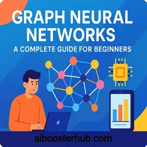
Graph Neural Networks: A Complete Guide for Beginners
Graph neural networks (GNNs) have emerged as one of the most powerful tools in deep learning, enabling AI systems to understand and learn from data that exists in graph structures. Unlike traditional neural networks that work with grid-like data such as images or sequences, GNNs can process complex relational data found in social networks, molecules, knowledge graphs, and recommendation systems.
This comprehensive guide provides a gentle introduction to graph neural networks, exploring their foundations, methods, and real-world applications.
1. Understanding graphs and why they matter
Before diving into graph neural networks, it’s essential to understand what graphs are and why they’re so prevalent in real-world data. A graph is a mathematical structure consisting of nodes (also called vertices) and edges that connect these nodes. Graphs can represent relationships between entities in ways that traditional data structures cannot.
What makes graph data special
Graph-structured data appears everywhere in our digital world. Social networks like Facebook and Twitter are graphs where users are nodes and friendships are edges. In biology, protein interaction networks are graphs that help scientists understand cellular processes. E-commerce platforms use graphs to model customer behavior and product relationships for recommendations.
The key advantage of graphs is their flexibility in representing irregular, non-Euclidean data. Unlike images that have a fixed grid structure or text that follows a sequential pattern, graphs can have varying numbers of neighbors for each node, no fixed ordering, and complex connectivity patterns. This flexibility makes graphs ideal for modeling real-world systems but also presents unique challenges for machine learning.
Types of graph learning tasks
Graph neural networks can tackle various types of problems depending on what we want to predict:
Node classification involves predicting properties or categories for individual nodes in a graph. For example, in a social network, we might want to identify users’ interests or detect spam accounts. In citation networks, node classification can categorize academic papers into research areas.
Graph classification treats entire graphs as input and assigns labels to them. This is crucial in chemistry where each molecule is represented as a graph, and we want to predict molecular properties like toxicity or drug effectiveness. Graph classification also appears in program analysis, where code structures are represented as graphs.
Link prediction aims to predict missing or future connections between nodes. Recommendation systems heavily rely on this task—predicting which products a user might like or which people they might want to connect with.
Graph generation involves creating entirely new graph structures, useful for designing new molecules in drug discovery or generating synthetic social networks for testing algorithms.
2. The foundation of graph neural networks
Graph neural networks extend traditional neural networks to operate on graph-structured data. The fundamental idea is to learn node representations by aggregating information from a node’s local neighborhood, similar to how convolutional neural networks aggregate information from nearby pixels.
The message passing framework
At the heart of most GNN architectures lies the message passing mechanism. This elegant framework consists of two key operations repeated across multiple layers:
- Message aggregation: Each node collects information from its neighbors
- Node update: Each node updates its representation based on aggregated messages
Mathematically, for a node \(v\) at layer \(k\), the update can be expressed as:
$$ \mathbf{h}_v^{(k)} = \text{UPDATE}^{(k)}\left(\mathbf{h}_v^{(k-1)}, \text{AGGREGATE}^{(k)}\left({\mathbf{h}_u^{(k-1)} : u \in \mathcal{N}(v)}\right)\right) $$
where \(\mathbf{h}_v^{(k)}\) is the representation of node \(v\) at layer \(k\), and \(\mathcal{N}(v)\) denotes the neighbors of node \(v\).
This process allows information to propagate through the graph structure. After \(k\) layers, each node’s representation captures information from nodes up to \(k\) hops away in the graph.
How powerful are graph neural networks
The expressive power of GNNs—their ability to distinguish different graph structures—has been rigorously studied. Research has shown that standard message passing GNNs have the same discriminative power as the Weisfeiler-Lehman graph isomorphism test, a classical algorithm for testing if two graphs are identical.
However, this also reveals limitations. There exist non-isomorphic graphs that GNNs cannot distinguish, which has motivated research into more powerful architectures. Understanding these theoretical foundations helps practitioners choose appropriate GNN architectures for their specific problems.
3. Popular GNN architectures: a review of methods and applications
The field of graph deep learning has produced numerous GNN variants, each with unique strengths. This section provides a comprehensive survey on graph neural networks architectures that have proven most effective.
Graph Convolutional Networks (GCN)
Graph Convolutional Networks introduced a spectral approach to graph learning that has become foundational. The GCN layer performs a normalized aggregation of neighbor features:
$$ \mathbf{H}^{(k+1)} = \sigma\left(\tilde{\mathbf{D}}^{-1/2}\tilde{\mathbf{A}}\tilde{\mathbf{D}}^{-1/2}\mathbf{H}^{(k)}\mathbf{W}^{(k)}\right) $$
where \(\tilde{\mathbf{A}} = \mathbf{A} + \mathbf{I}\) is the adjacency matrix with self-loops, \(\tilde{\mathbf{D}}\) is the degree matrix, \(\mathbf{W}^{(k)}\) is a learnable weight matrix, and \(\sigma\) is an activation function.
Here’s a simple Python implementation using PyTorch:
import torch
import torch.nn as nn
import torch.nn.functional as F

class GCNLayer(nn.Module):
    def __init__(self, in_features, out_features):
        super(GCNLayer, self).__init__()
        self.linear = nn.Linear(in_features, out_features)

    def forward(self, X, adj_matrix):
        """
        X: Node feature matrix (num_nodes, in_features)
        adj_matrix: Normalized adjacency matrix with self-loops
        """
        # Aggregate neighbor features
        aggregated = torch.mm(adj_matrix, X)
        # Apply linear transformation
        output = self.linear(aggregated)
        return F.relu(output)

class GCN(nn.Module):
    def __init__(self, num_features, hidden_dim, num_classes):
        super(GCN, self).__init__()
        self.conv1 = GCNLayer(num_features, hidden_dim)
        self.conv2 = GCNLayer(hidden_dim, num_classes)

    def forward(self, X, adj_matrix):
        X = self.conv1(X, adj_matrix)
        X = F.dropout(X, p=0.5, training=self.training)
        X = self.conv2(X, adj_matrix)
        return F.log_softmax(X, dim=1)
GraphSAGE: sampling and aggregating
GraphSAGE (Graph Sample and Aggregate) introduced a framework that samples a fixed-size neighborhood for each node, making it scalable to large graphs. Instead of using all neighbors, GraphSAGE samples a subset and applies various aggregation functions:
- Mean aggregator: Takes the element-wise mean of neighbor features
- LSTM aggregator: Treats neighbors as a sequence
- Pooling aggregator: Applies max pooling after element-wise transformations
This sampling approach makes GraphSAGE particularly suitable for inductive learning, where the model must generalize to unseen nodes.
Graph Attention Networks (GAT)
Graph Attention Networks introduced attention mechanisms to GNNs, allowing nodes to learn which neighbors are most important. The attention coefficient between nodes (i) and (j) is computed as:
$$\alpha_{ij} =
\frac{
\exp\Big(
\text{LeakyReLU}\big(\mathbf{a}^\top [\, \mathbf{W}\mathbf{h}_i \,\|\, \mathbf{W}\mathbf{h}_j ]\big)
\Big)
}{
\sum_{k \in \mathcal{N}(i)}
\exp\Big(
\text{LeakyReLU}\big(\mathbf{a}^\top [\, \mathbf{W}\mathbf{h}_i \,\|\, \mathbf{W}\mathbf{h}_k ]\big)
\Big)
}$$
This attention mechanism provides interpretability—we can visualize which connections the model considers important—and often improves performance on heterogeneous graphs where different edges carry different importance.
Graph Isomorphism Network (GIN)
The Graph Isomorphism Network was designed to maximize expressive power. GIN proved that by using a sum aggregation with an injective function, GNNs can be as powerful as the Weisfeiler-Lehman test:
$$\mathbf{h}_v^{(k)} =
\text{MLP}^{(k)}\left(
\big(1 + \epsilon^{(k)}\big) \cdot \mathbf{h}_v^{(k-1)}
+ \sum_{u \in \mathcal{N}(v)} \mathbf{h}_u^{(k-1)}
\right)$$
where \(\epsilon\) is a learnable parameter and MLP is a multi-layer perceptron. This architecture is particularly effective for graph classification tasks.
4. Training graph neural networks
Training GNNs presents unique challenges compared to traditional neural networks. Understanding these challenges and the techniques to address them is crucial for practical implementation.
Data preparation and graph construction
The first step is converting your problem into graph format. For node classification on existing graphs like social networks, this is straightforward. However, for other domains, you need to construct appropriate graph representations.
For image data, you might create graphs where pixels or image patches are nodes, connected based on spatial proximity. For text, you could build graphs connecting words or sentences based on syntactic or semantic relationships. In molecular applications, atoms become nodes and chemical bonds become edges.
Here’s an example of creating a simple graph dataset in Python:
import torch
from torch_geometric.data import Data

# Create a small graph with 4 nodes
# Node features (4 nodes, 3 features each)
x = torch.tensor([[1.0, 0.5, 0.2],
                  [0.8, 0.3, 0.9],
                  [0.4, 0.7, 0.1],
                  [0.9, 0.2, 0.6]], dtype=torch.float)

# Edge list (source, target)
edge_index = torch.tensor([[0, 1, 1, 2, 2, 3, 3, 0],
                           [1, 0, 2, 1, 3, 2, 0, 3]], dtype=torch.long)

# Node labels for classification
y = torch.tensor([0, 1, 0, 1], dtype=torch.long)

# Create graph data object
data = Data(x=x, edge_index=edge_index, y=y)

print(f"Number of nodes: {data.num_nodes}")
print(f"Number of edges: {data.num_edges}")
print(f"Graph features: {data.num_node_features}")
Loss functions and optimization
For node classification, cross-entropy loss is standard:
$$\mathcal{L} =
– \sum_{v \in \mathcal{V}_{\text{train}}}
\sum_{c=1}^{C}
y_{vc} \, \log\big(\hat{y}_{vc}\big) $$
where \(y_{vc}\) is the true label and \(\hat{y}_{vc}\) is the predicted probability for node \(v\) belonging to class \(c\).
For graph classification, you first need to obtain a graph-level representation, typically through a readout function that aggregates node representations:
def graph_readout(node_embeddings, batch_indices):
    """
    Aggregate node embeddings to graph-level representation
    node_embeddings: (num_nodes, embedding_dim)
    batch_indices: (num_nodes,) indicating which graph each node belongs to
    """
    # Sum pooling
    graph_embedding = torch.zeros(batch_indices.max() + 1,
                                   node_embeddings.size(1))
    graph_embedding.scatter_add_(0,
                                  batch_indices.unsqueeze(1).expand_as(node_embeddings),
                                  node_embeddings)
    return graph_embedding
Addressing over-smoothing and over-fitting
A significant challenge in GNNs is over-smoothing, where node representations become indistinguishable after many layers. This happens because repeated neighborhood aggregation makes distant nodes’ representations converge.
Solutions include:
- Limiting depth: Using fewer GNN layers (typically 2-4 layers)
- Residual connections: Adding skip connections similar to ResNets
- Normalization techniques: Applying batch normalization or layer normalization
- Dropout: Randomly dropping edges or nodes during training
For over-fitting, standard techniques apply: dropout, early stopping, and graph data augmentation (randomly removing edges, adding noise to features, or creating subgraphs).
5. Real-world applications and use cases
Graph neural networks have demonstrated remarkable success across diverse domains, transforming how we approach problems involving relational data.
Drug discovery and molecular property prediction
In pharmaceutical research, GNNs have become essential for predicting molecular properties. Molecules are naturally represented as graphs where atoms are nodes and bonds are edges. GNNs can predict toxicity, solubility, biological activity, and other properties crucial for drug development.
For example, predicting whether a molecule can bind to a specific protein target involves:
- Converting the molecular structure to a graph representation
- Encoding atom types, charges, and bond types as features
- Using a GNN to learn molecular representations
- Classifying binding affinity
This approach has accelerated virtual screening, allowing researchers to evaluate millions of compounds computationally before expensive laboratory testing.
Social network analysis
GNNs excel at understanding social dynamics. Applications include:
Community detection: Identifying groups of closely connected users Influence prediction: Determining which users are most influential in spreading information Recommendation systems: Predicting user preferences based on social connections and behavior patterns Fake account detection: Identifying suspicious accounts by analyzing connection patterns and behavior
The power of GNNs in social networks comes from their ability to capture both user features and the network structure simultaneously, leading to more accurate predictions than methods using either in isolation.
Knowledge graphs and reasoning
Knowledge graphs organize information as entities (nodes) and relationships (edges). GNNs enable:
Link prediction: Inferring missing facts in knowledge bases Entity classification: Categorizing entities based on their relationships Question answering: Reasoning over graph-structured knowledge to answer complex queries
Major technology companies use GNN-powered knowledge graphs to enhance search engines, power virtual assistants, and improve content understanding.
Traffic and transportation networks
Urban planning and traffic management leverage GNNs to model road networks. Applications include:
Traffic forecasting: Predicting congestion on road segments by modeling the road network as a graph where intersections are nodes Route optimization: Finding optimal paths considering real-time conditions Demand prediction: Forecasting ride-sharing or bike-sharing demand across a city
These systems must handle spatial dependencies (nearby locations affect each other) and temporal dynamics (traffic patterns change over time), often combining GNNs with recurrent or temporal networks.
Computer vision with graph structures
While images are traditionally processed with CNNs, GNNs offer advantages for tasks involving relationships between objects:
Scene graph generation: Creating structured representations of images showing objects and their relationships Point cloud processing: Learning from 3D point clouds by constructing k-nearest neighbor graphs Action recognition: Modeling human skeletons as graphs where joints are nodes and bones are edges
6. Implementing your first GNN project
Let’s build a complete node classification project using a real-world citation network, where papers cite each other and we want to predict research categories.
Step-by-step implementation
import torch
import torch.nn.functional as F
from torch_geometric.datasets import Planetoid
from torch_geometric.nn import GCNConv

# Step 1: Load dataset (Cora citation network)
dataset = Planetoid(root='/tmp/Cora', name='Cora')
data = dataset[0]

print(f"Number of nodes: {data.num_nodes}")
print(f"Number of edges: {data.num_edges}")
print(f"Number of features: {dataset.num_features}")
print(f"Number of classes: {dataset.num_classes}")

# Step 2: Define GNN model
class GCNClassifier(torch.nn.Module):
    def __init__(self, num_features, hidden_channels, num_classes):
        super(GCNClassifier, self).__init__()
        self.conv1 = GCNConv(num_features, hidden_channels)
        self.conv2 = GCNConv(hidden_channels, num_classes)
        self.dropout = torch.nn.Dropout(p=0.5)

    def forward(self, x, edge_index):
        # First GNN layer
        x = self.conv1(x, edge_index)
        x = F.relu(x)
        x = self.dropout(x)

        # Second GNN layer
        x = self.conv2(x, edge_index)
        return F.log_softmax(x, dim=1)

# Step 3: Initialize model and optimizer
model = GCNClassifier(
    num_features=dataset.num_features,
    hidden_channels=16,
    num_classes=dataset.num_classes
)
optimizer = torch.optim.Adam(model.parameters(), lr=0.01, weight_decay=5e-4)

# Step 4: Training function
def train():
    model.train()
    optimizer.zero_grad()
    out = model(data.x, data.edge_index)
    loss = F.nll_loss(out[data.train_mask], data.y[data.train_mask])
    loss.backward()
    optimizer.step()
    return loss.item()

# Step 5: Evaluation function
def evaluate():
    model.eval()
    with torch.no_grad():
        out = model(data.x, data.edge_index)
        pred = out.argmax(dim=1)

        train_correct = pred[data.train_mask] == data.y[data.train_mask]
        train_acc = int(train_correct.sum()) / int(data.train_mask.sum())

        test_correct = pred[data.test_mask] == data.y[data.test_mask]
        test_acc = int(test_correct.sum()) / int(data.test_mask.sum())

        return train_acc, test_acc

# Step 6: Training loop
for epoch in range(1, 201):
    loss = train()
    if epoch % 20 == 0:
        train_acc, test_acc = evaluate()
        print(f'Epoch: {epoch:03d}, Loss: {loss:.4f}, '
              f'Train Acc: {train_acc:.4f}, Test Acc: {test_acc:.4f}')
Best practices and tips
When implementing GNN projects, consider these guidelines:
Start simple: Begin with a basic architecture like GCN before trying more complex models. Often, simple models perform surprisingly well.
Monitor over-smoothing: If performance degrades with more layers, you’re likely experiencing over-smoothing. Try fewer layers or add residual connections.
Feature engineering matters: Good node features significantly impact performance. Domain knowledge helps create informative features.
Tune hyperparameters: Learning rate, hidden dimensions, dropout rate, and number of layers all affect performance. Use validation sets for tuning.
Handle imbalanced data: Many real-world graphs have imbalanced class distributions. Consider weighted loss functions or sampling strategies.
Scalability considerations: For large graphs, consider mini-batch training with sampling methods like those used in GraphSAGE.
7. Future directions and advanced topics
The field of graph deep learning continues to evolve rapidly, with exciting developments expanding what GNNs can achieve.
Heterogeneous graphs
Real-world graphs often contain multiple node types and edge types. Heterogeneous GNNs handle this complexity by learning type-specific transformations. For example, academic networks contain papers, authors, and venues, each with different features and relationships.
Dynamic and temporal graphs
Many real-world graphs change over time—social connections form and break, molecules undergo reactions, traffic patterns fluctuate. Temporal GNNs incorporate time by extending message passing to handle temporal sequences of graph snapshots or continuous-time interactions.
Graph transformers
Inspired by the success of transformers in NLP and vision, researchers are developing graph transformer architectures that use attention mechanisms to capture long-range dependencies in graphs more effectively than traditional message passing.
Explainability and interpretability
Understanding why a GNN makes specific predictions is crucial for applications like drug discovery and fraud detection. Techniques for explaining GNN predictions include attention visualization, gradient-based methods, and generating subgraph explanations.
Self-supervised learning on graphs
Training GNNs often requires labeled data, which is expensive to obtain. Self-supervised methods like contrastive learning, graph augmentation, and masked prediction enable learning useful representations from unlabeled graphs.