K-means clustering: Algorithm guide and applications
K-means clustering stands as one of the most popular and intuitive unsupervised machine learning algorithms. Whether you’re analyzing customer behavior, compressing images, or discovering patterns in complex datasets, understanding what is k means and how the k-means algorithm works is essential for any data scientist or AI practitioner. This comprehensive guide explores k-means clustering from fundamental concepts to practical implementations, helping you master this powerful clustering algorithm.

1. Understanding k-means clustering fundamentals
What is clustering in machine learning?
Clustering is an unsupervised learning technique that groups similar data points together based on their characteristics. Unlike supervised learning where we have labeled data, cluster analysis discovers hidden patterns without predefined categories. The goal is to maximize similarity within clusters while maximizing differences between clusters.
K-means clustering, often simply called kmeans, is a centroid-based algorithm that partitions data into k distinct clusters. Each cluster is represented by its centroid—the mean position of all points in that cluster. The algorithm iteratively refines these centroids until it achieves optimal grouping.
The k meaning in k-means
The “k” in k-means represents the number of clusters you want to identify in your dataset. This is a hyperparameter that you must specify before running the algorithm. For instance, if you’re segmenting customers into three groups, you would set k=3. Choosing the right k value is crucial for meaningful results, and we’ll explore techniques for this later.
How k-means differs from other clustering algorithms
While hierarchical clustering builds a tree-like structure of nested clusters, k-means assigns each data point to exactly one cluster. Hierarchical clustering doesn’t require you to specify the number of clusters upfront, but k means clustering algorithm is generally faster and more scalable for large datasets. Other clustering algorithms like DBSCAN focus on density, whereas k-means uses distance from centroids as its primary metric.
2. The k-means clustering algorithm explained
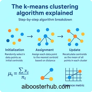
Step-by-step algorithm breakdown
The k means algorithm follows an elegant iterative process:
- Initialization: Randomly select k data points as initial centroids
- Assignment: Assign each data point to the nearest centroid based on distance
- Update: Recalculate centroids as the mean of all points in each cluster
- Repeat: Continue steps 2-3 until centroids no longer change significantly or maximum iterations are reached
This process guarantees convergence, though not necessarily to the global optimum. The algorithm minimizes the within-cluster sum of squares (WCSS), also known as inertia.
Mathematical foundation
The objective function that k-means clustering minimizes is:
$$J = \sum_{i=1}^{k} \sum_{x \in C_i} ||x – \mu_i||^2$$
Where:
- \(k\) is the number of clusters
- \(C_i\) represents cluster \(i\)
- \(x\) is a data point in cluster \(C_i\)
- \(\mu_i\) is the centroid of cluster \(C_i\)
- \(||x – \mu_i||^2\) is the squared Euclidean distance
Calculating the average position of points within each cluster defines what we mean by ‘means’ in this context. The centroid update formula is:
$$\mu_i = \frac{1}{|C_i|} \sum_{x \in C_i} x$$
Distance metrics in k-means
While Euclidean distance is the default metric, understanding distance measurement is critical. Euclidean distance between points \(p\) and \(q\) in n-dimensional space is:
$$d(p,q) = \sqrt{\sum_{i=1}^{n} (p_i – q_i)^2}$$
Alternative distance metrics like Manhattan distance or cosine similarity can be used for specific applications, though they require modifications to the standard k means cluster algorithm.
3. Implementing k-means clustering in Python
Basic implementation with scikit-learn
Let’s start with a practical implementation using Python’s scikit-learn library:
import numpy as np
import matplotlib.pyplot as plt
from sklearn.cluster import KMeans
from sklearn.datasets import make_blobs

# Generate sample data
X, y_true = make_blobs(n_samples=300, centers=4,
                       cluster_std=0.60, random_state=42)

# Apply k-means clustering
kmeans = KMeans(n_clusters=4, random_state=42, n_init=10)
y_kmeans = kmeans.fit_predict(X)

# Visualize results
plt.figure(figsize=(10, 6))
plt.scatter(X[:, 0], X[:, 1], c=y_kmeans, s=50, cmap='viridis')
plt.scatter(kmeans.cluster_centers_[:, 0],
           kmeans.cluster_centers_[:, 1],
           c='red', s=200, alpha=0.75, marker='X')
plt.title('K-Means Clustering Results')
plt.xlabel('Feature 1')
plt.ylabel('Feature 2')
plt.show()

print(f"Inertia: {kmeans.inertia_:.2f}")
print(f"Cluster centers:\n{kmeans.cluster_centers_}")
Building k-means from scratch
Understanding the algorithm deeply requires implementing it yourself:
class KMeansFromScratch:
    def __init__(self, n_clusters=3, max_iters=100, random_state=42):
        self.n_clusters = n_clusters
        self.max_iters = max_iters
        self.random_state = random_state

    def fit(self, X):
        np.random.seed(self.random_state)
        # Random initialization
        random_indices = np.random.choice(X.shape[0],
                                         self.n_clusters,
                                         replace=False)
        self.centroids = X[random_indices]

        for iteration in range(self.max_iters):
            # Assignment step
            distances = self._calculate_distances(X)
            labels = np.argmin(distances, axis=1)

            # Update step
            new_centroids = np.array([X[labels == k].mean(axis=0)
                                     for k in range(self.n_clusters)])

            # Check convergence
            if np.allclose(self.centroids, new_centroids):
                break

            self.centroids = new_centroids

        return labels

    def _calculate_distances(self, X):
        distances = np.zeros((X.shape[0], self.n_clusters))
        for k in range(self.n_clusters):
            distances[:, k] = np.linalg.norm(X - self.centroids[k], axis=1)
        return distances

# Test the implementation
kmeans_custom = KMeansFromScratch(n_clusters=4, random_state=42)
labels_custom = kmeans_custom.fit(X)
Handling real-world data
When working with actual datasets, preprocessing is crucial:
from sklearn.preprocessing import StandardScaler
from sklearn.decomposition import PCA
import pandas as pd

# Load and prepare data
def prepare_data_for_clustering(df, features):
    # Handle missing values
    df_clean = df[features].dropna()

    # Standardize features
    scaler = StandardScaler()
    X_scaled = scaler.fit_transform(df_clean)

    return X_scaled, scaler

# Example with dimensionality reduction
def cluster_with_pca(X, n_clusters=3, n_components=2):
    # Apply PCA for visualization
    pca = PCA(n_components=n_components)
    X_pca = pca.fit_transform(X)

    # Perform clustering
    kmeans = KMeans(n_clusters=n_clusters, random_state=42)
    labels = kmeans.fit_predict(X_pca)

    print(f"Explained variance: {pca.explained_variance_ratio_}")

    return labels, X_pca, kmeans
4. Determining the optimal number of clusters
This technique plots
An elbow method plots inertia against different k values. The “elbow” point where the rate of decrease sharply shifts indicates the optimal k:
def elbow_method(X, max_k=10):
    inertias = []
    K_range = range(1, max_k + 1)

    for k in K_range:
        kmeans = KMeans(n_clusters=k, random_state=42, n_init=10)
        kmeans.fit(X)
        inertias.append(kmeans.inertia_)

    # Plot the elbow curve
    plt.figure(figsize=(10, 6))
    plt.plot(K_range, inertias, 'bo-')
    plt.xlabel('Number of Clusters (k)')
    plt.ylabel('Inertia (WCSS)')
    plt.title('Elbow Method for Optimal k')
    plt.grid(True)
    plt.show()

    return inertias

# Apply elbow method
elbow_method(X, max_k=10)
Silhouette analysis
The silhouette score measures how similar a point is to its own cluster compared to other clusters. Values range from -1 to 1, where higher is better:
from sklearn.metrics import silhouette_score, silhouette_samples
import matplotlib.cm as cm

def silhouette_analysis(X, k_range):
    silhouette_scores = []

    for k in k_range:
        kmeans = KMeans(n_clusters=k, random_state=42)
        labels = kmeans.fit_predict(X)
        score = silhouette_score(X, labels)
        silhouette_scores.append(score)
        print(f"k={k}, Silhouette Score: {score:.3f}")

    # Plot silhouette scores
    plt.figure(figsize=(10, 6))
    plt.plot(k_range, silhouette_scores, 'go-')
    plt.xlabel('Number of Clusters (k)')
    plt.ylabel('Silhouette Score')
    plt.title('Silhouette Analysis')
    plt.grid(True)
    plt.show()

    return silhouette_scores

# Perform silhouette analysis
silhouette_analysis(X, range(2, 11))
Gap statistic method
The gap statistic compares the total intracluster variation for different k values with their expected values under null reference distribution:
def gap_statistic(X, k_range, n_refs=10):
    gaps = []

    for k in k_range:
        # Cluster original data
        kmeans = KMeans(n_clusters=k, random_state=42)
        kmeans.fit(X)
        original_inertia = kmeans.inertia_

        # Generate reference datasets and cluster them
        ref_inertias = []
        for _ in range(n_refs):
            random_data = np.random.uniform(X.min(axis=0),
                                           X.max(axis=0),
                                           size=X.shape)
            kmeans_ref = KMeans(n_clusters=k, random_state=42)
            kmeans_ref.fit(random_data)
            ref_inertias.append(np.log(kmeans_ref.inertia_))

        gap = np.mean(ref_inertias) - np.log(original_inertia)
        gaps.append(gap)

    return gaps
5. Advanced techniques and optimizations
K-means++ initialization
Standard k-means can converge to poor local optima depending on initial centroid placement. K-means++ improves initialization by selecting centroids that are far apart:
from sklearn.cluster import KMeans

# K-means++ is the default in scikit-learn
kmeans_plus = KMeans(n_clusters=4, init='k-means++',
                     n_init=10, random_state=42)
labels = kmeans_plus.fit_predict(X)
The k-means++ algorithm selects initial centroids with probability proportional to their squared distance from the nearest existing centroid, improving convergence speed and quality.
Mini-batch k-means for large datasets
When dealing with massive datasets, mini-batch k-means offers significant speedup:
from sklearn.cluster import MiniBatchKMeans
import time

# Generate large dataset
X_large, _ = make_blobs(n_samples=100000, centers=5,
                        cluster_std=1.0, random_state=42)

# Standard k-means
start_time = time.time()
kmeans_standard = KMeans(n_clusters=5, random_state=42)
kmeans_standard.fit(X_large)
standard_time = time.time() - start_time

# Mini-batch k-means
start_time = time.time()
kmeans_minibatch = MiniBatchKMeans(n_clusters=5,
                                   batch_size=1000,
                                   random_state=42)
kmeans_minibatch.fit(X_large)
minibatch_time = time.time() - start_time

print(f"Standard K-Means: {standard_time:.2f}s")
print(f"Mini-Batch K-Means: {minibatch_time:.2f}s")
print(f"Speedup: {standard_time/minibatch_time:.2fx")
Handling categorical and mixed data
K-means works best with numerical data, but we can adapt it for categorical features:
from sklearn.preprocessing import OneHotEncoder

def kmeans_mixed_data(df, numerical_features, categorical_features, n_clusters):
    # One-hot encode categorical features
    encoder = OneHotEncoder(sparse=False, drop='first')
    cat_encoded = encoder.fit_transform(df[categorical_features])

    # Standardize numerical features
    scaler = StandardScaler()
    num_scaled = scaler.fit_transform(df[numerical_features])

    # Combine features
    X_combined = np.hstack([num_scaled, cat_encoded])

    # Apply k-means
    kmeans = KMeans(n_clusters=n_clusters, random_state=42)
    labels = kmeans.fit_predict(X_combined)

    return labels, kmeans
6. Real-world applications of k-means clustering
Customer segmentation in marketing
One of the most popular applications is segmenting customers based on purchasing behavior:
# Example: Customer segmentation
def customer_segmentation_analysis(customer_data):
    # Select relevant features
    features = ['annual_income', 'spending_score',
                'age', 'purchase_frequency']

    # Prepare data
    X_scaled, scaler = prepare_data_for_clustering(customer_data, features)

    # Determine optimal clusters
    silhouette_scores = silhouette_analysis(X_scaled, range(2, 8))

    # Apply k-means with optimal k
    optimal_k = 4
    kmeans = KMeans(n_clusters=optimal_k, random_state=42)
    customer_data['segment'] = kmeans.fit_predict(X_scaled)

    # Analyze segments
    segment_profiles = customer_data.groupby('segment')[features].mean()
    print("\nSegment Profiles:")
    print(segment_profiles)

    return customer_data, kmeans
Image compression and color quantization
K-means clustering can compress images by reducing the number of colors:
from sklearn.cluster import KMeans
from PIL import Image

def compress_image_kmeans(image_path, n_colors=16):
    # Load image
    img = Image.open(image_path)
    img_array = np.array(img)

    # Reshape to 2D array of pixels
    h, w, d = img_array.shape
    pixels = img_array.reshape(-1, d)

    # Apply k-means
    kmeans = KMeans(n_clusters=n_colors, random_state=42)
    labels = kmeans.fit_predict(pixels)

    # Replace each pixel with its cluster center
    compressed_pixels = kmeans.cluster_centers_[labels]
    compressed_img = compressed_pixels.reshape(h, w, d).astype(np.uint8)

    # Calculate compression ratio
    original_colors = len(np.unique(pixels, axis=0))
    print(f"Original colors: {original_colors}")
    print(f"Compressed to: {n_colors} colors")

    return compressed_img
Anomaly detection
Points far from any cluster center can be identified as anomalies:
def detect_anomalies_kmeans(X, contamination=0.1):
    # Apply k-means
    kmeans = KMeans(n_clusters=3, random_state=42)
    kmeans.fit(X)

    # Calculate distances to nearest centroid
    distances = np.min(kmeans.transform(X), axis=1)

    # Set threshold based on contamination
    threshold = np.percentile(distances, 100 * (1 - contamination))

    # Identify anomalies
    anomalies = distances > threshold

    print(f"Detected {np.sum(anomalies)} anomalies")

    return anomalies, distances
Document clustering and text analysis
K-means clustering helps organize large document collections:
from sklearn.feature_extraction.text import TfidfVectorizer

def cluster_documents(documents, n_clusters=5):
    # Convert documents to TF-IDF vectors
    vectorizer = TfidfVectorizer(max_features=1000,
                                 stop_words='english')
    X_tfidf = vectorizer.fit_transform(documents)

    # Apply k-means
    kmeans = KMeans(n_clusters=n_clusters, random_state=42)
    labels = kmeans.fit_predict(X_tfidf)

    # Get top terms per cluster
    feature_names = vectorizer.get_feature_names_out()
    for i in range(n_clusters):
        center = kmeans.cluster_centers_[i]
        top_indices = center.argsort()[-10:][::-1]
        top_terms = [feature_names[idx] for idx in top_indices]
        print(f"\nCluster {i}: {', '.join(top_terms)}")

    return labels, kmeans
7. Limitations and best practices
Understanding k-means limitations
While powerful, kmeans clustering has important constraints:
- Assumes spherical clusters: K-means struggles with elongated or irregularly shaped clusters
- Sensitive to outliers: Extreme values can significantly skew centroids
- Requires k specification: You must choose the number of clusters beforehand
- Scale dependent: Features with larger ranges dominate distance calculations
- Local optima: Different initializations can yield different results
When to use alternatives
Consider hierarchical clustering when you need a dendrogram showing relationships between clusters, or when you’re unsure about k. For density-based clusters of arbitrary shape, DBSCAN or HDBSCAN may be more appropriate. For very high-dimensional data, spectral clustering can be more effective.
Best practices for k-means clustering
- Always standardize features: Use StandardScaler to ensure all features contribute equally
- Try multiple initializations: Use n_init parameter to run k-means multiple times
- Validate results: Use multiple metrics (silhouette, elbow, gap statistic) to choose k
- Handle outliers: Consider removing or treating outliers before clustering
- Visualize results: Use dimensionality reduction (PCA, t-SNE) to visualize clusters
- Domain knowledge matters: Interpret clusters in the context of your problem
- Test sensitivity: Check how results change with different k values
# Complete pipeline with best practices
def robust_kmeans_pipeline(X, k_range=range(2, 11)):
    # Standardize features
    scaler = StandardScaler()
    X_scaled = scaler.fit_transform(X)

    # Remove outliers using IQR method
    Q1 = np.percentile(X_scaled, 25, axis=0)
    Q3 = np.percentile(X_scaled, 75, axis=0)
    IQR = Q3 - Q1
    outlier_mask = ~((X_scaled < (Q1 - 1.5 * IQR)) |
                     (X_scaled > (Q3 + 1.5 * IQR))).any(axis=1)
    X_clean = X_scaled[outlier_mask]

    # Find optimal k
    silhouette_scores = []
    inertias = []

    for k in k_range:
        kmeans = KMeans(n_clusters=k, n_init=20, random_state=42)
        labels = kmeans.fit_predict(X_clean)
        silhouette_scores.append(silhouette_score(X_clean, labels))
        inertias.append(kmeans.inertia_)

    # Select optimal k based on silhouette score
    optimal_k = k_range[np.argmax(silhouette_scores)]
    print(f"Optimal k: {optimal_k}")

    # Final clustering
    final_kmeans = KMeans(n_clusters=optimal_k, n_init=20, random_state=42)
    final_labels = final_kmeans.fit_predict(X_clean)

    return final_labels, final_kmeans, scaler