Linear Regression in Machine Learning: Python, Scikit-Learn
Linear regression stands as one of the foundational pillars of machine learning and statistical modeling. Despite its simplicity, this powerful algorithm continues to be widely used across industries for predictive analytics, trend forecasting, and understanding relationships between variables. Whether you’re predicting house prices, analyzing sales trends, or modeling scientific phenomena, linear regression in machine learning provides an intuitive yet effective approach to supervised learning problems.

In this comprehensive guide, we’ll explore everything from the mathematical foundations to practical implementation using Python and scikit-learn, ensuring you gain both theoretical understanding and hands-on expertise.
1. What is linear regression in machine learning?
Understanding the fundamentals
Linear regression is a supervised machine learning algorithm that models the relationship between one or more input features (independent variables) and a continuous output variable (dependent variable). The core idea is to find the best-fitting straight line—or hyperplane in higher dimensions—that describes how the output changes as inputs vary.
The term “regression” in machine learning refers to predicting continuous numerical values, distinguishing it from classification tasks that predict discrete categories. Linear regression assumes this relationship can be approximated by a linear function, making it both interpretable and computationally efficient.
The mathematical foundation
At its heart, linear regression seeks to model the relationship using the equation:
$$y = \beta_0 + \beta_1x_1 + \beta_2x_2 + … + \beta_nx_n + \epsilon$$
Where:
- \(y\) is the predicted output
- \(\beta_0\) is the intercept (bias term)
- \(\beta_1, \beta_2, …, \beta_n\) are the coefficients (weights)
- \(x_1, x_2, …, x_n\) are the input features
- \(\epsilon\) represents the error term
For simple linear regression with a single feature, this simplifies to:
$$y = \beta_0 + \beta_1x$$
This represents a straight line where \(\beta_0\) is the y-intercept and \(\beta_1\) is the slope.
Types of linear regression
Simple linear regression involves one independent variable predicting one dependent variable. For example, predicting a person’s weight based solely on their height.
Multiple linear regression extends this concept to multiple independent variables. For instance, predicting house prices based on square footage, number of bedrooms, location, and age of the property.
2. How linear regression works
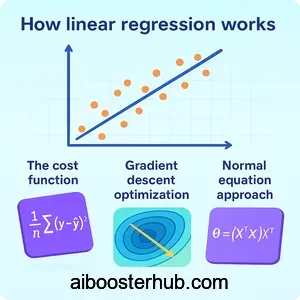
The cost function
Linear regression in machine learning works by finding the optimal parameters that minimize the difference between predicted and actual values. This difference is quantified using a cost function, typically the Mean Squared Error (MSE):
$$J(\beta) = \frac{1}{2m}\sum_{i=1}^{m}(h_{\beta}(x^{(i)}) – y^{(i)})^2$$
Where:
- \(m\) is the number of training examples
- \(h_{\beta}(x^{(i)})\) is the predicted value for the \(i\)-th example
- \(y^{(i)}\) is the actual value
- \(\beta\) represents all parameters (coefficients)
The goal is to find parameter values that minimize this cost function, resulting in predictions that are as close as possible to the actual values.
Gradient descent optimization
Gradient descent is an iterative optimization algorithm used to find the minimum of the cost function. It updates parameters in the direction that reduces the cost:
$$\beta_j := \beta_j – \alpha\frac{\partial}{\partial\beta_j}J(\beta)$$
Where \(\alpha\) is the learning rate, controlling the step size of each iteration. The algorithm continues until convergence, where further iterations produce minimal improvement.
Normal equation approach
An alternative to gradient descent is the normal equation, which provides a closed-form solution by solving for parameters analytically:
$$\beta = (X^TX)^{-1}X^Ty$$
This method directly computes the optimal parameters in one step, though it can be computationally expensive for large datasets due to matrix inversion.
3. Implementing linear regression python
Setting up your environment
Before diving into implementation, ensure you have the necessary libraries installed. Python’s ecosystem provides powerful tools for machine learning, with scikit-learn being the go-to library for regression in ml tasks.
import numpy as np
import pandas as pd
import matplotlib.pyplot as plt
from sklearn.model_selection import train_test_split
from sklearn.linear_model import LinearRegression
from sklearn.metrics import mean_squared_error, r2_score
Creating a simple dataset
Let’s start with a practical example: predicting student test scores based on hours studied.
# Generate sample data
np.random.seed(42)
hours_studied = np.array([1, 2, 3, 4, 5, 6, 7, 8, 9, 10]).reshape(-1, 1)
test_scores = 50 + 5 * hours_studied.flatten() + np.random.randn(10) * 3

# Visualize the data
plt.scatter(hours_studied, test_scores, color='blue', label='Actual scores')
plt.xlabel('Hours Studied')
plt.ylabel('Test Score')
plt.title('Student Test Scores vs Study Hours')
plt.legend()
plt.show()
Building your first model with sklearn linear regression
The sklearn.linear_model module provides the LinearRegression class, making implementation straightforward:
# Create and train the model
model = LinearRegression()
model.fit(hours_studied, test_scores)

# Make predictions
predictions = model.predict(hours_studied)

# Display model parameters
print(f"Intercept (β₀): {model.intercept_:.2f}")
print(f"Coefficient (β₁): {model.coef_[0]:.2f}")

# Visualize the regression line
plt.scatter(hours_studied, test_scores, color='blue', label='Actual scores')
plt.plot(hours_studied, predictions, color='red', linewidth=2, label='Regression line')
plt.xlabel('Hours Studied')
plt.ylabel('Test Score')
plt.title('Linear Regression: Study Hours vs Test Scores')
plt.legend()
plt.show()
The LinearRegression object automatically computes the optimal parameters using the normal equation method by default, providing a simple interface for regression in machine learning tasks.
4. Multiple linear regression with scikit learn
Working with multiple features
Real-world problems rarely involve just one predictor variable. Let’s extend our example to predict house prices using multiple features:
# Create a dataset with multiple features
data = {
    'square_feet': [1500, 1600, 1700, 1800, 1900, 2000, 2100, 2200, 2300, 2400],
    'bedrooms': [3, 3, 3, 4, 4, 4, 4, 5, 5, 5],
    'age_years': [10, 8, 12, 5, 6, 3, 8, 2, 4, 1],
    'price': [300000, 320000, 310000, 360000, 370000, 400000, 390000, 430000, 440000, 470000]
}

df = pd.DataFrame(data)

# Prepare features and target
X = df[['square_feet', 'bedrooms', 'age_years']]
y = df['price']

# Split data into training and testing sets
X_train, X_test, y_train, y_test = train_test_split(X, y, test_size=0.2, random_state=42)

# Train the model
multi_model = LinearRegression()
multi_model.fit(X_train, y_train)

# Display coefficients
print("Model Coefficients:")
for feature, coef in zip(X.columns, multi_model.coef_):
    print(f"  {feature}: {coef:.2f}")
print(f"Intercept: {multi_model.intercept_:.2f}")
Feature interpretation
The coefficients in multiple linear regression tell us how much the output changes for a one-unit increase in each feature, holding other features constant. In our house price example:
- A positive coefficient for square_feet indicates larger homes cost more
- The bedrooms coefficient shows the price change per additional bedroom
- A negative age_years coefficient suggests older homes are less expensive
This interpretability makes linear regression sklearn implementations valuable for understanding feature importance and business insights.
Making predictions on new data
# Predict on test set
y_pred = multi_model.predict(X_test)

# Predict for a new house
new_house = [[2000, 4, 5]]  # 2000 sq ft, 4 bedrooms, 5 years old
predicted_price = multi_model.predict(new_house)
print(f"\nPredicted price for new house: ${predicted_price[0]:,.2f}")
5. Evaluating model performance
Key metrics for sklearn regression
Evaluating how well your linear regression model performs is crucial for understanding its reliability and limitations. Several metrics help quantify model accuracy:
Mean Squared Error (MSE)
MSE measures the average squared difference between predicted and actual values:
$$MSE = \frac{1}{m}\sum_{i=1}^{m}(y_i – \hat{y}_i)^2$$
mse = mean_squared_error(y_test, y_pred)
print(f"Mean Squared Error: {mse:,.2f}")
Root Mean Squared Error (RMSE)
RMSE is the square root of MSE, providing error in the same units as the target variable:
rmse = np.sqrt(mse)
print(f"Root Mean Squared Error: ${rmse:,.2f}")
R-squared (Coefficient of Determination)
R² indicates the proportion of variance in the dependent variable explained by the independent variables:
$$R^2 = 1 – \frac{\sum_{i=1}^{m} (y_i – \hat{y}_i)^2}{\sum_{i=1}^{m} (y_i – \bar{y})^2}$$
r2 = r2_score(y_test, y_pred)
print(f"R² Score: {r2:.4f}")
An R² value closer to 1 indicates better model fit, while values near 0 suggest the model explains little variance.
Residual analysis
Examining residuals (differences between actual and predicted values) helps identify patterns that violate linear regression assumptions:
# Calculate residuals
residuals = y_test - y_pred

# Plot residuals
plt.figure(figsize=(10, 4))

plt.subplot(1, 2, 1)
plt.scatter(y_pred, residuals, alpha=0.7)
plt.axhline(y=0, color='r', linestyle='--')
plt.xlabel('Predicted Values')
plt.ylabel('Residuals')
plt.title('Residual Plot')

plt.subplot(1, 2, 2)
plt.hist(residuals, bins=10, edgecolor='black')
plt.xlabel('Residuals')
plt.ylabel('Frequency')
plt.title('Residual Distribution')

plt.tight_layout()
plt.show()
Ideally, residuals should be randomly scattered around zero with no clear patterns, indicating the model captures the relationship appropriately.
6. Advanced techniques and considerations
Feature scaling and normalization
When features have different scales, those with larger values can dominate the model. Standardization ensures all features contribute proportionally:
from sklearn.preprocessing import StandardScaler

# Scale features
scaler = StandardScaler()
X_train_scaled = scaler.fit_transform(X_train)
X_test_scaled = scaler.transform(X_test)

# Train model on scaled data
scaled_model = LinearRegression()
scaled_model.fit(X_train_scaled, y_train)
y_pred_scaled = scaled_model.predict(X_test_scaled)

print(f"R² with scaled features: {r2_score(y_test, y_pred_scaled):.4f}")
Polynomial features
Linear regression can model non-linear relationships by transforming features into polynomial terms:
from sklearn.preprocessing import PolynomialFeatures

# Create polynomial features
poly = PolynomialFeatures(degree=2, include_bias=False)
X_poly = poly.fit_transform(hours_studied)

# Train polynomial regression
poly_model = LinearRegression()
poly_model.fit(X_poly, test_scores)

# Visualize polynomial fit
X_plot = np.linspace(1, 10, 100).reshape(-1, 1)
X_plot_poly = poly.transform(X_plot)
y_plot = poly_model.predict(X_plot_poly)

plt.scatter(hours_studied, test_scores, color='blue', label='Data')
plt.plot(X_plot, y_plot, color='red', label='Polynomial fit')
plt.xlabel('Hours Studied')
plt.ylabel('Test Score')
plt.legend()
plt.show()
Regularization techniques
Regularization prevents overfitting by penalizing large coefficients. Scikit-learn provides Ridge (L2) and Lasso (L1) regression:
from sklearn.linear_model import Ridge, Lasso

# Ridge regression
ridge_model = Ridge(alpha=1.0)
ridge_model.fit(X_train_scaled, y_train)
y_pred_ridge = ridge_model.predict(X_test_scaled)

# Lasso regression
lasso_model = Lasso(alpha=0.1)
lasso_model.fit(X_train_scaled, y_train)
y_pred_lasso = lasso_model.predict(X_test_scaled)

print(f"Ridge R²: {r2_score(y_test, y_pred_ridge):.4f}")
print(f"Lasso R²: {r2_score(y_test, y_pred_lasso):.4f}")
Comparing with other tools
While we’ve focused on python linear regression with scikit-learn, other tools exist for regression analysis. The linregress python function from scipy.stats provides basic statistical linear regression for simple cases:
from scipy.stats import linregress

slope, intercept, r_value, p_value, std_err = linregress(hours_studied.flatten(), test_scores)
print(f"Slope: {slope:.2f}, Intercept: {intercept:.2f}, R²: {r_value**2:.4f}")
For MATLAB users, linear regression matlab implementations offer similar functionality through built-in functions, though Python’s scikit-learn provides a more comprehensive machine learning ecosystem.
7. Best practices and common pitfalls
Assumptions of linear regression
Linear regression in ml relies on several key assumptions:
- Linearity: The relationship between features and target is linear
- Independence: Observations are independent of each other
- Homoscedasticity: Residuals have constant variance across all levels of predictors
- Normality: Residuals are normally distributed
- No multicollinearity: Independent variables are not highly correlated
Violating these assumptions can lead to unreliable predictions and incorrect interpretations.
Handling outliers and missing data
Outliers can significantly impact regression results. Consider removing extreme outliers or using robust regression techniques:
# Identify outliers using z-score
from scipy import stats

z_scores = np.abs(stats.zscore(df[['price']]))
df_clean = df[(z_scores < 3).all(axis=1)]
For missing data, imputation strategies or removing incomplete records may be necessary before training your sklearn regression model.
Avoiding overfitting
Overfitting occurs when a model learns noise in training data rather than true patterns. Strategies to prevent this include:
- Using train-test splits or cross-validation
- Applying regularization (Ridge, Lasso)
- Reducing feature count through selection
- Gathering more training data
from sklearn.model_selection import cross_val_score

# Perform cross-validation
cv_scores = cross_val_score(multi_model, X, y, cv=5, scoring='r2')
print(f"Cross-validation R² scores: {cv_scores}")
print(f"Mean CV R²: {cv_scores.mean():.4f} (+/- {cv_scores.std() * 2:.4f})")