LSTM vs GRU: Key Differences Explained

Recurrent neural networks have revolutionized how machines process sequential data, from natural language to time series forecasting. Among the most powerful RNN architectures are Long Short Term Memory (LSTM) and Gated Recurrent Unit (GRU) networks. Both architectures solve the vanishing gradient problem that plagued traditional RNNs, but they do so in distinctly different ways. Understanding these differences is crucial for choosing the right model for your deep learning project.

Content

1. Understanding recurrent neural networks

What makes RNNs special

Recurrent neural networks differ fundamentally from traditional feedforward neural networks in their ability to maintain memory. While standard neural networks treat each input independently, an RNN model processes sequences by maintaining an internal state that captures information from previous inputs. This makes RNNs ideal for tasks where context and order matter—like speech recognition, machine translation, and sentiment analysis.

The basic RNN architecture contains a hidden state that gets updated at each time step. When processing a sequence, the network takes both the current input and the previous hidden state to produce an output and update its memory. Mathematically, this can be expressed as:

$$h_t = \tanh(W_{hh}h_{t-1} + W_{xh}x_t + b_h)$$

$$y_t = W_{hy}h_t + b_y$$

Where $h_t$ represents the hidden state at time (t), $x_t$ is the input, and $y_t$ is the output.

The vanishing gradient problem

Despite their elegant design, traditional RNNs struggle with long-term dependencies. When training on sequences, gradients must flow backward through time. As these gradients propagate through many time steps, they tend to either explode or vanish exponentially. The vanishing gradient problem is particularly severe—gradients can shrink to near zero, making it nearly impossible for the network to learn relationships between events separated by many time steps.

Consider a simple example: understanding the sentence “The cat, which was sitting on the mat that my grandmother knitted last winter, was hungry.” To correctly process “was hungry,” the network needs to remember “cat” from much earlier in the sequence. Traditional RNNs often fail at such tasks because the gradient signal from “hungry” becomes too weak to affect the weights related to “cat.”

Enter gating mechanisms

The solution to vanishing gradients came through gating mechanisms—learnable filters that control information flow through the network. Gates can selectively remember or forget information, creating shortcut paths for gradients to flow backward through time. This innovation led to two dominant architectures: the LSTM neural network and the Gated Recurrent Unit.

2. Deep dive into LSTM networks

The LSTM architecture

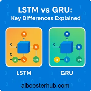
Long Short Term Memory networks, introduced by Hochreiter and Schmidhuber, employ a sophisticated gating system with three gates: forget gate, input gate, and output gate. The LSTM network also maintains two separate states: a cell state (long-term memory) and a hidden state (short-term memory).

The cell state acts as a highway for information, allowing gradients to flow with minimal transformation. Gates regulate what information gets added to or removed from this cell state.

Here’s how each gate functions:

Forget Gate: Decides what information to discard from the cell state.

$$f_t = \sigma(W_f \cdot [h_{t-1}, x_t] + b_f)$$

Input Gate: Determines what new information to store in the cell state.

$$i_t = \sigma(W_i \cdot [h_{t-1}, x_t] + b_i)$$

$$\tilde{C}_t = \tanh(W_C \cdot [h_{t-1}, x_t] + b_C)$$

Cell State Update: Combines forget and input gate outputs.

$$C_t = f_t * C_{t-1} + i_t * \tilde{C}_t$$

Output Gate: Controls what information from the cell state to output.

$$o_t = \sigma(W_o \cdot [h_{t-1}, x_t] + b_o)$$

$$h_t = o_t * \tanh(C_t)$$

Where $\sigma$ represents the sigmoid activation function, and $*$ denotes element-wise multiplication.

How LSTM processes sequences

Let’s walk through a concrete example. Imagine processing the text “The weather is sunny” for sentiment analysis. At each word:

The forget gate evaluates whether previous context remains relevant
The input gate decides how much the current word should update the memory
The cell state gets updated by forgetting old information and adding new information
The output gate determines what aspects of the updated memory to use for prediction

When processing “sunny,” the LSTM might strongly activate the input gate (this word carries sentiment information), partially activate the forget gate (some earlier context remains relevant), and activate the output gate (we need this information for the final prediction).

Implementing LSTM in Python

Here’s a practical implementation using PyTorch:

import torch
import torch.nn as nn

class LSTMModel(nn.Module):
    def __init__(self, input_size, hidden_size, num_layers, output_size):
        super(LSTMModel, self).__init__()
        self.hidden_size = hidden_size
        self.num_layers = num_layers
        
        # LSTM layer
        self.lstm = nn.LSTM(input_size, hidden_size, num_layers, 
                           batch_first=True)
        
        # Fully connected output layer
        self.fc = nn.Linear(hidden_size, output_size)
    
    def forward(self, x):
        # Initialize hidden and cell states
        h0 = torch.zeros(self.num_layers, x.size(0), 
                        self.hidden_size).to(x.device)
        c0 = torch.zeros(self.num_layers, x.size(0), 
                        self.hidden_size).to(x.device)
        
        # Forward propagate LSTM
        out, _ = self.lstm(x, (h0, c0))
        
        # Get output from the last time step
        out = self.fc(out[:, -1, :])
        return out

# Example usage for time series prediction
input_size = 1      # One feature per time step
hidden_size = 50    # Hidden state dimension
num_layers = 2      # Stacked LSTM layers
output_size = 1     # Predict one value

model = LSTMModel(input_size, hidden_size, num_layers, output_size)
print(model)

Bidirectional LSTM

A powerful variant is the bidirectional LSTM, which processes sequences in both forward and backward directions. This bidirectional RNN architecture captures context from both past and future, making it excellent for tasks where the entire sequence is available upfront, like text classification or named entity recognition.

class BiLSTMModel(nn.Module):
    def __init__(self, input_size, hidden_size, num_layers, output_size):
        super(BiLSTMModel, self).__init__()
        
        # Bidirectional LSTM
        self.lstm = nn.LSTM(input_size, hidden_size, num_layers,
                           batch_first=True, bidirectional=True)
        
        # Note: hidden_size * 2 because bidirectional
        self.fc = nn.Linear(hidden_size * 2, output_size)
    
    def forward(self, x):
        out, _ = self.lstm(x)
        out = self.fc(out[:, -1, :])
        return out

In this bidirectional configuration, each time step’s output contains information from both directions, providing richer context for predictions.

3. Understanding GRU networks

The simplified gating approach

The Gated Recurrent Unit was introduced as a simpler alternative to the LSTM architecture. GRU networks achieve similar performance with fewer parameters by consolidating LSTM’s three gates into two: a reset gate and an update gate. Additionally, GRU eliminates the separate cell state, using only a hidden state.

This simplification reduces computational complexity while maintaining the ability to capture long-term dependencies. The GRU architecture has become particularly popular in applications where training efficiency matters.

GRU mathematical formulation

The GRU operates through these equations:

Reset Gate: Determines how much past information to forget.

$$r_t = \sigma(W_r \cdot [h_{t-1}, x_t] + b_r)$$

Update Gate: Decides how much past information to keep and how much new information to add.

$$z_t = \sigma(W_z \cdot [h_{t-1}, x_t] + b_z)$$

Candidate Hidden State: Computes new memory content.

$$\tilde{h}_t = \tanh(W_h \cdot [r_t \cdot h_{t-1}, x_t] + b_h)$$

Final Hidden State: Interpolates between previous and candidate hidden states.

$$h_t = (1 – z_t) * h_{t-1} + z_t * \tilde{h}_t$$

Notice how the update gate $z_t$ performs double duty—it simultaneously controls forgetting old information (via $1 – z_t$) and adding new information (via $z_t$).

How GRU differs in operation

Let’s revisit our sentiment analysis example with “The weather is sunny.” Processing through a GRU:

The reset gate determines which parts of previous context to use when computing new memory
New candidate memory is computed, incorporating selectively reset past information
The update gate decides how to balance old memory with new candidate memory
The hidden state is directly updated and used for output

When processing “sunny,” if the update gate activates strongly, the GRU heavily weights this new sentiment-bearing word while de-emphasizing previous neutral words.

Implementing GRU in Python

Here’s a GRU implementation in PyTorch:

class GRUModel(nn.Module):
    def __init__(self, input_size, hidden_size, num_layers, output_size):
        super(GRUModel, self).__init__()
        self.hidden_size = hidden_size
        self.num_layers = num_layers
        
        # GRU layer
        self.gru = nn.GRU(input_size, hidden_size, num_layers,
                         batch_first=True)
        
        # Fully connected output layer
        self.fc = nn.Linear(hidden_size, output_size)
    
    def forward(self, x):
        # Initialize hidden state
        h0 = torch.zeros(self.num_layers, x.size(0),
                        self.hidden_size).to(x.device)
        
        # Forward propagate GRU
        out, _ = self.gru(x, h0)
        
        # Get output from the last time step
        out = self.fc(out[:, -1, :])
        return out

# Example usage
model = GRUModel(input_size=1, hidden_size=50, 
                num_layers=2, output_size=1)
print(model)

The GRU implementation is notably simpler—we only need to initialize one hidden state instead of both hidden and cell states.

4. Key differences between LSTM and GRU

Architectural complexity

The most obvious difference lies in complexity. LSTM networks employ three gates (forget, input, output) and maintain two separate states (cell state and hidden state). This results in more parameters to learn. Specifically, an LSTM has four sets of weights per layer, while GRU has three.

For a layer with input dimension (n) and hidden dimension (h):

LSTM parameters: $4 \times (n \times h + h \times h + h)$
GRU parameters: $3 \times (n \times h + h \times h + h)$

This means GRU is approximately 25% more parameter-efficient.

Memory mechanism

LSTM’s dual-state system provides explicit separation between long-term memory (cell state) and short-term working memory (hidden state). The cell state can flow through time with minimal modification, acting as a memory highway.

GRU merges these concepts into a single hidden state. The update gate in GRU controls memory in a more direct way—it literally interpolates between old and new memory. This simplification works surprisingly well in practice.

Training speed and efficiency

Due to fewer parameters and simpler computations, GRU networks typically train faster than LSTM networks. This advantage becomes significant with large datasets or when rapid experimentation is needed. For resource-constrained environments like mobile devices or edge computing, GRU’s efficiency is particularly valuable.

Here’s a benchmark comparison:

import time
import torch
import torch.nn as nn

def benchmark_model(model, input_tensor, iterations=1000):
    model.eval()
    start_time = time.time()
    
    with torch.no_grad():
        for _ in range(iterations):
            _ = model(input_tensor)
    
    end_time = time.time()
    return end_time - start_time

# Create test input
sequence_length = 100
batch_size = 32
input_size = 10
input_tensor = torch.randn(batch_size, sequence_length, input_size)

# Initialize models
lstm_model = nn.LSTM(input_size, 128, num_layers=2, batch_first=True)
gru_model = nn.GRU(input_size, 128, num_layers=2, batch_first=True)

# Benchmark
lstm_time = benchmark_model(lstm_model, input_tensor)
gru_time = benchmark_model(gru_model, input_tensor)

print(f"LSTM inference time: {lstm_time:.4f} seconds")
print(f"GRU inference time: {gru_time:.4f} seconds")
print(f"Speedup: {lstm_time/gru_time:.2f}x")

Typically, GRU shows 15-30% faster inference times.

Performance on different tasks

Performance comparisons show task-dependent results. LSTM networks often excel at tasks requiring precise long-term memory and complex temporal patterns, like music generation or complex language modeling. The separate cell state provides fine-grained control over what information to maintain.

GRU networks perform competitively on many sequence tasks, particularly those with shorter dependencies or where training efficiency matters. They’ve shown excellent results in machine translation, speech recognition, and time series forecasting.

Gradient flow characteristics

Both architectures address vanishing gradients, but differently. LSTM’s cell state provides a nearly uninterrupted gradient highway, while GRU’s update gate creates adaptive gradient paths. In practice, both handle long sequences well, though LSTM’s mechanism is theoretically more robust for extremely long sequences.

Practical comparison

Here’s a side-by-side training example:

import torch
import torch.nn as nn
import torch.optim as optim
from torch.utils.data import DataLoader, TensorDataset

# Generate synthetic sequence data
def generate_data(num_samples, seq_length, input_size):
    X = torch.randn(num_samples, seq_length, input_size)
    # Simple target: sum of sequence
    y = torch.sum(X, dim=1).mean(dim=1, keepdim=True)
    return X, y

# Training function
def train_model(model, train_loader, epochs=10):
    criterion = nn.MSELoss()
    optimizer = optim.Adam(model.parameters(), lr=0.001)
    
    for epoch in range(epochs):
        total_loss = 0
        for batch_X, batch_y in train_loader:
            optimizer.zero_grad()
            outputs = model(batch_X)
            loss = criterion(outputs, batch_y)
            loss.backward()
            optimizer.step()
            total_loss += loss.item()
        
        print(f"Epoch {epoch+1}/{epochs}, Loss: {total_loss/len(train_loader):.4f}")

# Generate data
X, y = generate_data(1000, 50, 10)
dataset = TensorDataset(X, y)
train_loader = DataLoader(dataset, batch_size=32, shuffle=True)

# Train LSTM
print("Training LSTM:")
lstm_model = LSTMModel(10, 64, 2, 1)
train_model(lstm_model, train_loader)

# Train GRU
print("\nTraining GRU:")
gru_model = GRUModel(10, 64, 2, 1)
train_model(gru_model, train_loader)

5. When to use LSTM vs GRU

Choose LSTM when:

Complex long-term dependencies matter: If your task requires remembering specific information over very long sequences (hundreds or thousands of time steps), LSTM’s explicit memory cell provides better control. Natural language processing tasks like document-level sentiment analysis or long-form text generation benefit from this capability.

You have sufficient computational resources: When training time and computational power aren’t constraints, LSTM’s additional parameters can capture more nuanced patterns. Large-scale production systems with dedicated GPU clusters can leverage LSTM’s full potential.

Fine-grained memory control is needed: Tasks requiring precise control over what to remember and forget—like complex music generation where multiple simultaneous patterns must be tracked—benefit from LSTM’s separate gates.

Bidirectional processing adds value: Bidirectional LSTM excels at tasks where the entire sequence is available, like named entity recognition or question answering, where context from both directions enriches understanding.

Choose GRU when:

Training efficiency is important: When you need to iterate quickly or train on limited hardware, GRU’s faster training and lower memory footprint make it ideal. This is particularly valuable during the experimental phase of projects.

The dataset is limited: With fewer parameters, GRU is less prone to overfitting on smaller datasets. If you’re working with thousands rather than millions of samples, GRU often generalizes better.

Real-time inference matters: Applications requiring low-latency predictions—like real-time speech recognition or live translation—benefit from GRU’s faster inference speed.

Moderate sequence lengths prevail: For sequences of tens to hundreds of time steps (the range of many practical applications), GRU performs comparably to LSTM while being more efficient.

Hybrid approaches

Sometimes the best solution combines both architectures. You might use:

Stacked architectures: GRU layers for initial feature extraction followed by LSTM layers for final processing
Ensemble methods: Training both LSTM and GRU models and combining their predictions
Architecture search: Using automated methods to discover optimal combinations for specific tasks

class HybridModel(nn.Module):
    def __init__(self, input_size, hidden_size, output_size):
        super(HybridModel, self).__init__()
        
        # First layer: GRU for efficient feature extraction
        self.gru = nn.GRU(input_size, hidden_size, batch_first=True)
        
        # Second layer: LSTM for refined sequence modeling
        self.lstm = nn.LSTM(hidden_size, hidden_size, batch_first=True)
        
        self.fc = nn.Linear(hidden_size, output_size)
    
    def forward(self, x):
        # GRU processing
        gru_out, _ = self.gru(x)
        
        # LSTM processing
        lstm_out, _ = self.lstm(gru_out)
        
        # Final prediction
        out = self.fc(lstm_out[:, -1, :])
        return out

6. Practical considerations for RNN deep learning

Preprocessing and input preparation

Both LSTM and GRU require careful data preparation. Sequences should be normalized to prevent gradient issues. For text data, embedding layers transform discrete tokens into continuous vectors:

class TextClassifier(nn.Module):
    def __init__(self, vocab_size, embed_dim, hidden_size, num_classes):
        super(TextClassifier, self).__init__()
        
        # Embedding layer
        self.embedding = nn.Embedding(vocab_size, embed_dim)
        
        # RNN layer (choose LSTM or GRU)
        self.rnn = nn.GRU(embed_dim, hidden_size, batch_first=True)
        
        # Output layer
        self.fc = nn.Linear(hidden_size, num_classes)
        self.dropout = nn.Dropout(0.5)
    
    def forward(self, x):
        # Convert token indices to embeddings
        embedded = self.embedding(x)
        
        # Process through RNN
        rnn_out, _ = self.rnn(embedded)
        
        # Apply dropout and classify
        out = self.dropout(rnn_out[:, -1, :])
        out = self.fc(out)
        return out

Handling variable-length sequences

Real-world data rarely comes in uniform lengths. PyTorch provides packing utilities:

from torch.nn.utils.rnn import pack_padded_sequence, pad_packed_sequence

class VariableLengthRNN(nn.Module):
    def __init__(self, input_size, hidden_size, output_size):
        super(VariableLengthRNN, self).__init__()
        self.lstm = nn.LSTM(input_size, hidden_size, batch_first=True)
        self.fc = nn.Linear(hidden_size, output_size)
    
    def forward(self, x, lengths):
        # Pack padded sequences
        packed = pack_padded_sequence(x, lengths, batch_first=True, 
                                     enforce_sorted=False)
        
        # Process through LSTM
        packed_out, _ = self.lstm(packed)
        
        # Unpack
        output, _ = pad_packed_sequence(packed_out, batch_first=True)
        
        # Use actual last time steps
        last_outputs = output[range(len(lengths)), lengths - 1]
        return self.fc(last_outputs)

Regularization techniques

Both LSTM and GRU can overfit. Common regularization strategies include:

Dropout: Apply between RNN layers and before the output layer Recurrent dropout: Drop connections within the recurrent layer Weight decay: L2 regularization on parameters Gradient clipping: Prevent exploding gradients

# Dropout in RNN
model = nn.LSTM(input_size, hidden_size, num_layers=2, 
               dropout=0.3, batch_first=True)

# Gradient clipping during training
torch.nn.utils.clip_grad_norm_(model.parameters(), max_norm=1.0)

Optimization tips

Learning rate scheduling: Start with higher learning rates and decay over time Batch normalization: Can stabilize training, though less common in RNNs Attention mechanisms: Enhance both LSTM and GRU by allowing them to focus on relevant parts of the input sequence

class AttentionRNN(nn.Module):
    def __init__(self, input_size, hidden_size, output_size):
        super(AttentionRNN, self).__init__()
        self.lstm = nn.LSTM(input_size, hidden_size, batch_first=True)
        self.attention = nn.Linear(hidden_size, 1)
        self.fc = nn.Linear(hidden_size, output_size)
    
    def forward(self, x):
        lstm_out, _ = self.lstm(x)
        
        # Compute attention weights
        attention_weights = torch.softmax(
            self.attention(lstm_out), dim=1
        )
        
        # Apply attention
        context = torch.sum(attention_weights * lstm_out, dim=1)
        
        return self.fc(context)

7. Conclusion

The choice between LSTM and GRU ultimately depends on your specific use case. LSTM networks provide sophisticated memory management through their three-gate architecture and dual-state system, making them ideal for complex sequential tasks with long-term dependencies. GRU networks offer a streamlined alternative with faster training and comparable performance for many applications, particularly when efficiency matters.

Rather than viewing these architectures as competitors, consider them complementary tools in your deep learning toolkit. Start with GRU for rapid prototyping and switch to LSTM when you need additional modeling capacity. Both have proven their worth across countless applications in natural language processing, time series analysis, and beyond. By understanding the fundamental differences in their gating mechanisms and memory systems, you can make informed decisions that balance performance, efficiency, and practical constraints. The recurrent neural network family continues to evolve, but LSTM and GRU remain foundational architectures that every AI practitioner should master.

Explore more:

LSTM vs GRU: Key Differences Explained