Multiple Linear Regression: Models, Analysis & Applications Explained

Multiple linear regression stands as one of the most powerful yet accessible statistical techniques for analyzing relationships between variables. Whether you’re predicting house prices based on multiple features, forecasting sales from various marketing channels, or building the foundation for more complex AI models, multiple linear regression serves as an essential tool in your analytical arsenal.

This comprehensive guide will walk you through everything you need to know about multiple linear regression—from its theoretical foundations to practical implementation. By the end of this article, you’ll understand not just what a regression model is, but how to build, interpret, and apply multivariate linear regression to solve real-world problems.

Content

1. Understanding regression analysis: The foundation

What is regression analysis?

Regression analysis is a statistical method used to examine the relationship between one dependent variable and one or more independent variables. At its core, regression analysis helps us answer questions like: “How does a change in X affect Y?” or “Can we predict Y based on the values of X?”

To understand what is a regression analysis, think of it as drawing a line (or surface) through data points that best represents the relationship between variables. This line allows us to make predictions about unknown values and understand which factors most significantly influence our outcome of interest.

What is a regression model?

A regression model is the mathematical representation of the relationship between variables. The regression model meaning encompasses both the equation that describes this relationship and the assumptions underlying it. In essence, regression models serve as a bridge between observed data and predictions about future or unknown values.

There are various types of regression models, each suited to different scenarios:

Simple linear regression: Models the relationship between one independent variable and one dependent variable
Multiple linear regression: Extends simple regression to include multiple independent variables
Polynomial regression: Captures non-linear relationships using polynomial terms
Logistic regression: Used for binary classification problems

Why multiple linear regression matters in AI

Multiple linear regression forms the conceptual backbone of many machine learning algorithms. While deep learning dominates headlines, linear regression models remain invaluable for:

Interpretability: Unlike black-box models, multiple regression analysis provides clear insights into how each variable influences predictions
Baseline modeling: It establishes performance benchmarks for more complex algorithms
Feature importance: Identifies which variables matter most in your predictions
Computational efficiency: Trains quickly even on large datasets
Foundation building: Understanding multivariate linear regression is essential before tackling advanced ML concepts

2. The mathematics behind multiple linear regression

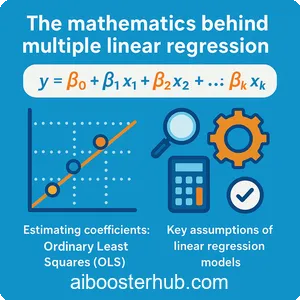
The multiple linear regression model equation

The multiple linear regression model expresses the relationship between a dependent variable (y) and multiple independent variables (x_1, x_2, …, x_p) as:

$$y = \beta_0 + \beta_1x_1 + \beta_2x_2 + … + \beta_px_p + \epsilon$$

Where:

$y$ is the dependent variable (what we’re trying to predict)
$x_1, x_2, …, x_p$ are the independent variables (predictors or features)
$\beta_0$ is the intercept (the value of $y$ when all\ (x\) variables equal zero)
$\beta_1, \beta_2, …, \beta_p$ are the coefficients (slopes) for each independent variable
$\epsilon$ is the error term (residual), representing unexplained variation

In matrix notation, this becomes more elegant:

$$\mathbf{y} = \mathbf{X}\boldsymbol{\beta} + \boldsymbol{\epsilon}$$

Where $\mathbf{y}$ is an $n \times 1$ vector of observations, $\mathbf{X}$ is an $n \times (p+1)$ design matrix, and $\boldsymbol{\beta}$ is a $(p+1) \times 1$ vector of coefficients.

Estimating coefficients: Ordinary Least Squares (OLS)

The most common method for estimating the coefficients in a linear regression model is Ordinary Least Squares (OLS). This method minimizes the sum of squared residuals:

$$\text{Minimize: } \sum_{i=1}^{n} (y_i – \hat{y}_i)^2 = \sum_{i=1}^{n} (y_i – (\beta_0 + \beta_1 x_{i1} + \dots + \beta_p x_{ip}))^2$$

The OLS solution can be expressed in matrix form as:

$$\hat{\boldsymbol{\beta}} = (\mathbf{X}^T\mathbf{X})^{-1}\mathbf{X}^T\mathbf{y}$$

This formula provides the coefficient estimates that minimize prediction error on the training data.

Key assumptions of linear regression models

For a multiple linear regression model to produce reliable results, several assumptions must hold:

Linearity: The relationship between independent and dependent variables is linear
Independence: Observations are independent of each other
Homoscedasticity: The variance of residuals is constant across all levels of independent variables
Normality: Residuals are normally distributed
No multicollinearity: Independent variables are not highly correlated with each other

Violating these assumptions can lead to biased estimates, incorrect standard errors, and unreliable predictions.

3. Building your first multiple linear regression model

Data preparation and exploration

Before building any regression model, thorough data preparation is essential. Let’s work through a practical example predicting house prices based on multiple features.

import numpy as np
import pandas as pd
import matplotlib.pyplot as plt
import seaborn as sns
from sklearn.model_selection import train_test_split
from sklearn.linear_model import LinearRegression
from sklearn.metrics import mean_squared_error, r2_score

# Create a synthetic dataset for house prices
np.random.seed(42)
n_samples = 500

# Features: square footage, number of bedrooms, age of house, distance to city center
square_footage = np.random.uniform(800, 3500, n_samples)
bedrooms = np.random.randint(1, 6, n_samples)
age = np.random.uniform(0, 50, n_samples)
distance_km = np.random.uniform(1, 30, n_samples)

# Generate price with some realistic relationships
price = (150 * square_footage + 
         20000 * bedrooms - 
         500 * age - 
         2000 * distance_km + 
         50000 + 
         np.random.normal(0, 30000, n_samples))

# Create DataFrame
df = pd.DataFrame({
    'square_footage': square_footage,
    'bedrooms': bedrooms,
    'age': age,
    'distance_km': distance_km,
    'price': price
})

# Display basic statistics
print(df.describe())
print("\nCorrelation Matrix:")
print(df.corr())

Training the multiple linear regression model

Now let’s build our multivariate linear regression model using Python’s scikit-learn library:

# Separate features and target
X = df[['square_footage', 'bedrooms', 'age', 'distance_km']]
y = df['price']

# Split data into training and testing sets
X_train, X_test, y_train, y_test = train_test_split(
    X, y, test_size=0.2, random_state=42
)

# Create and train the model
model = LinearRegression()
model.fit(X_train, y_train)

# Display the coefficients
print("Intercept:", model.intercept_)
print("\nCoefficients:")
for feature, coef in zip(X.columns, model.coef_):
    print(f"{feature}: {coef:.2f}")

Making predictions

Once trained, we can use our regression model to make predictions:

# Make predictions on test set
y_pred = model.predict(X_test)

# Example prediction for a specific house
new_house = np.array([[2000, 3, 10, 5]])  # 2000 sq ft, 3 bed, 10 years old, 5km from city
predicted_price = model.predict(new_house)
print(f"\nPredicted price for new house: ${predicted_price[0]:,.2f}")

# Visualize predictions vs actual values
plt.figure(figsize=(10, 6))
plt.scatter(y_test, y_pred, alpha=0.5)
plt.plot([y_test.min(), y_test.max()], [y_test.min(), y_test.max()], 
         'r--', lw=2, label='Perfect prediction')
plt.xlabel('Actual Price')
plt.ylabel('Predicted Price')
plt.title('Multiple Linear Regression: Predicted vs Actual Prices')
plt.legend()
plt.tight_layout()
plt.show()

4. Evaluating multiple regression analysis performance

Key performance metrics

Evaluating a regression model requires multiple metrics to assess different aspects of performance:

R-squared ((R^2)): Represents the proportion of variance in the dependent variable explained by the independent variables.

$$R^2 = 1 – \frac{\sum_{i=1}^{n} (y_i – \hat{y}_i)^2}{\sum_{i=1}^{n} (y_i – \bar{y})^2}$$

Values range from 0 to 1, with higher values indicating better fit.

Adjusted R-squared: Accounts for the number of predictors in the model, preventing overfitting:

$$R^2_{adj} = 1 – \frac{(1-R^2)(n-1)}{n-p-1}$$

Mean Squared Error (MSE): Average of squared differences between predicted and actual values:

$$MSE = \frac{1}{n}\sum_{i=1}^{n}(y_i – \hat{y}_i)^2$$

Root Mean Squared Error (RMSE): Square root of MSE, in the same units as the target variable:

$$RMSE = \sqrt{MSE}$$

Let’s calculate these metrics for our model:

# Calculate performance metrics
r2 = r2_score(y_test, y_pred)
mse = mean_squared_error(y_test, y_pred)
rmse = np.sqrt(mse)

# Calculate adjusted R-squared
n = len(y_test)
p = X_test.shape[1]
adjusted_r2 = 1 - (1 - r2) * (n - 1) / (n - p - 1)

print(f"R-squared: {r2:.4f}")
print(f"Adjusted R-squared: {adjusted_r2:.4f}")
print(f"Mean Squared Error: {mse:,.2f}")
print(f"Root Mean Squared Error: {rmse:,.2f}")

Residual analysis

Analyzing residuals (the differences between predicted and actual values) helps verify that our model meets the assumptions of linear regression:

# Calculate residuals
residuals = y_test - y_pred

# Create residual plots
fig, axes = plt.subplots(2, 2, figsize=(14, 10))

# Residuals vs Predicted Values
axes[0, 0].scatter(y_pred, residuals, alpha=0.5)
axes[0, 0].axhline(y=0, color='r', linestyle='--')
axes[0, 0].set_xlabel('Predicted Values')
axes[0, 0].set_ylabel('Residuals')
axes[0, 0].set_title('Residuals vs Predicted Values')

# Histogram of Residuals
axes[0, 1].hist(residuals, bins=30, edgecolor='black')
axes[0, 1].set_xlabel('Residuals')
axes[0, 1].set_ylabel('Frequency')
axes[0, 1].set_title('Distribution of Residuals')

# Q-Q Plot
from scipy import stats
stats.probplot(residuals, dist="norm", plot=axes[1, 0])
axes[1, 0].set_title('Q-Q Plot')

# Residuals vs Order
axes[1, 1].scatter(range(len(residuals)), residuals, alpha=0.5)
axes[1, 1].axhline(y=0, color='r', linestyle='--')
axes[1, 1].set_xlabel('Observation Order')
axes[1, 1].set_ylabel('Residuals')
axes[1, 1].set_title('Residuals vs Order')

plt.tight_layout()
plt.show()

Statistical significance testing

Understanding which predictors are statistically significant helps refine your model:

from scipy import stats

# Calculate standard errors and t-statistics
# This is a simplified calculation - statsmodels provides more comprehensive statistics
predictions = model.predict(X_train)
residuals_train = y_train - predictions
mse_train = np.mean(residuals_train**2)
n_train = len(y_train)
p_vars = X_train.shape[1]

# Degrees of freedom
df = n_train - p_vars - 1

# Print interpretation
print("Variable Importance:")
for feature, coef in zip(X.columns, model.coef_):
    print(f"\n{feature}:")
    print(f"  Coefficient: {coef:.2f}")
    print(f"  Interpretation: A 1-unit increase in {feature} is associated with a "
          f"${coef:.2f} change in price, holding other variables constant")

5. Advanced techniques in multiple linear regression

Feature engineering and transformation

Often, raw features need transformation to improve model performance. Common techniques include:

Polynomial features: Capture non-linear relationships

from sklearn.preprocessing import PolynomialFeatures

# Create polynomial features
poly = PolynomialFeatures(degree=2, include_bias=False)
X_poly = poly.fit_transform(X_train[['square_footage', 'age']])

# Train model with polynomial features
model_poly = LinearRegression()
model_poly.fit(X_poly, y_train)

print(f"Features created: {poly.get_feature_names_out(['square_footage', 'age'])}")

Interaction terms: Model how variables work together

# Create interaction term manually
X_train_interaction = X_train.copy()
X_train_interaction['sqft_bedrooms'] = X_train['square_footage'] * X_train['bedrooms']

X_test_interaction = X_test.copy()
X_test_interaction['sqft_bedrooms'] = X_test['square_footage'] * X_test['bedrooms']

# Train model with interaction
model_interaction = LinearRegression()
model_interaction.fit(X_train_interaction, y_train)

Feature scaling: Standardize features to similar ranges

from sklearn.preprocessing import StandardScaler

# Standardize features
scaler = StandardScaler()
X_train_scaled = scaler.fit_transform(X_train)
X_test_scaled = scaler.transform(X_test)

# Train model on scaled data
model_scaled = LinearRegression()
model_scaled.fit(X_train_scaled, y_train)

Handling multicollinearity

Multicollinearity occurs when independent variables are highly correlated, leading to unstable coefficient estimates. Detect it using:

Variance Inflation Factor (VIF):

from statsmodels.stats.outliers_influence import variance_inflation_factor

# Calculate VIF for each feature
vif_data = pd.DataFrame()
vif_data["Feature"] = X.columns
vif_data["VIF"] = [variance_inflation_factor(X.values, i) for i in range(X.shape[1])]

print("\nVariance Inflation Factors:")
print(vif_data)
print("\nRule of thumb: VIF > 10 indicates high multicollinearity")

Regularization: Ridge and Lasso regression

Regularization techniques help prevent overfitting and handle multicollinearity:

Ridge Regression (L2 regularization):

from sklearn.linear_model import Ridge

# Ridge regression with cross-validation to find best alpha
from sklearn.linear_model import RidgeCV

alphas = np.logspace(-3, 3, 100)
ridge_cv = RidgeCV(alphas=alphas, cv=5)
ridge_cv.fit(X_train, y_train)

print(f"Best alpha: {ridge_cv.alpha_}")
print(f"Ridge R-squared: {ridge_cv.score(X_test, y_test):.4f}")

Lasso Regression (L1 regularization):

from sklearn.linear_model import Lasso, LassoCV

# Lasso can perform feature selection by shrinking coefficients to zero
lasso_cv = LassoCV(alphas=alphas, cv=5, random_state=42)
lasso_cv.fit(X_train, y_train)

print(f"\nBest alpha: {lasso_cv.alpha_}")
print(f"Lasso R-squared: {lasso_cv.score(X_test, y_test):.4f}")

# Check which features were selected
print("\nFeature coefficients:")
for feature, coef in zip(X.columns, lasso_cv.coef_):
    print(f"{feature}: {coef:.2f}")

6. Real-world applications of multiple linear regression

Financial forecasting

Multiple regression analysis is extensively used in finance for:

Stock price prediction: Using market indicators, trading volumes, and economic factors
Credit scoring: Predicting loan default risk based on borrower characteristics
Portfolio optimization: Analyzing returns based on multiple asset classes

# Example: Simple stock return prediction
# Note: This is illustrative - real financial modeling requires much more sophistication

# Simulated financial data
np.random.seed(42)
n_days = 1000

market_return = np.random.normal(0.05, 0.15, n_days)
interest_rate = np.random.uniform(0.01, 0.05, n_days)
vix_index = np.random.uniform(10, 40, n_days)
sector_performance = np.random.normal(0.03, 0.12, n_days)

# Stock return influenced by multiple factors
stock_return = (0.8 * market_return + 
                -0.5 * interest_rate + 
                -0.01 * vix_index + 
                0.3 * sector_performance + 
                np.random.normal(0, 0.05, n_days))

# Build regression model
financial_df = pd.DataFrame({
    'market_return': market_return,
    'interest_rate': interest_rate,
    'vix': vix_index,
    'sector_perf': sector_performance,
    'stock_return': stock_return
})

X_fin = financial_df[['market_return', 'interest_rate', 'vix', 'sector_perf']]
y_fin = financial_df['stock_return']

model_fin = LinearRegression()
model_fin.fit(X_fin, y_fin)

print("Financial Model Coefficients:")
for feature, coef in zip(X_fin.columns, model_fin.coef_):
    print(f"{feature}: {coef:.4f}")

Marketing and business analytics

Businesses leverage multivariate linear regression for:

Sales forecasting: Predicting sales based on advertising spend, seasonality, and economic conditions
Customer lifetime value: Estimating long-term customer value from behavioral data
Pricing optimization: Understanding how price changes affect demand

# Example: Marketing mix modeling
np.random.seed(42)
n_weeks = 100

tv_spend = np.random.uniform(1000, 10000, n_weeks)
digital_spend = np.random.uniform(500, 5000, n_weeks)
print_spend = np.random.uniform(200, 2000, n_weeks)
seasonality = np.sin(np.linspace(0, 4*np.pi, n_weeks)) * 5000

# Sales influenced by marketing channels with diminishing returns
sales = (3 * np.sqrt(tv_spend) + 
         4 * np.sqrt(digital_spend) + 
         1.5 * np.sqrt(print_spend) + 
         seasonality + 
         10000 + 
         np.random.normal(0, 1000, n_weeks))

marketing_df = pd.DataFrame({
    'tv_spend': tv_spend,
    'digital_spend': digital_spend,
    'print_spend': print_spend,
    'sales': sales
})

# For linear model, we might use log transformation for diminishing returns
X_mkt = np.log1p(marketing_df[['tv_spend', 'digital_spend', 'print_spend']])
y_mkt = marketing_df['sales']

model_mkt = LinearRegression()
model_mkt.fit(X_mkt, y_mkt)

print("\nMarketing Mix Model - ROI Analysis:")
print(f"R-squared: {model_mkt.score(X_mkt, y_mkt):.4f}")

Healthcare and medical research

The healthcare industry uses regression models for:

Disease progression prediction: Modeling disease severity based on patient characteristics
Treatment efficacy analysis: Comparing treatment outcomes across patient groups
Resource allocation: Predicting hospital admissions and resource needs

Environmental science and sustainability

Environmental researchers apply linear regression analysis to:

Climate modeling: Predicting temperature changes from multiple environmental factors
Pollution analysis: Understanding sources and impacts of air quality
Energy consumption: Forecasting energy demand based on weather and demographics

7. Best practices and common pitfalls

Best practices for robust regression modeling

Start with exploratory data analysis: Understand your data distribution, outliers, and relationships before modeling
Check assumptions systematically: Verify linearity, independence, homoscedasticity, and normality
Use cross-validation: Don’t rely solely on test set performance; use k-fold cross-validation for robust estimates
Feature selection matters: More features doesn’t always mean better models; select meaningful predictors
Document your process: Keep track of transformations, assumptions, and decisions
Consider domain knowledge: Statistical significance doesn’t always mean practical significance

Common mistakes to avoid

Overfitting: Using too many features relative to sample size

# Use cross-validation to detect overfitting
from sklearn.model_selection import cross_val_score

cv_scores = cross_val_score(model, X, y, cv=5, 
                           scoring='r2')
print(f"Cross-validation R² scores: {cv_scores}")
print(f"Mean CV R²: {cv_scores.mean():.4f} (+/- {cv_scores.std() * 2:.4f})")

Extrapolation: Making predictions outside the range of training data

Ignoring outliers: Outliers can dramatically affect regression coefficients

Assuming causation: Correlation in regression doesn’t imply causation

When to use (and not use) multiple linear regression

Use multiple linear regression when:

Relationships are approximately linear
You need interpretable results
You have sufficient sample size (rule of thumb: at least 10-20 observations per predictor)
Independence assumption holds

Consider alternatives when:

Relationships are clearly non-linear (try polynomial regression, GAMs, or tree-based methods)
Target variable is categorical (use logistic regression or classification algorithms)
Data has complex interactions (consider neural networks or ensemble methods)
Dealing with time series (use ARIMA, LSTM, or specialized time series models)

8. Conclusion

Multiple linear regression remains one of the most valuable tools in the data scientist’s toolkit. While AI continues to advance with sophisticated deep learning architectures, the interpretability, efficiency, and theoretical foundation of regression models make them indispensable for both beginners and experienced practitioners.

The power of multiple linear regression lies not in its complexity, but in its elegant simplicity and remarkable versatility. Start applying these techniques to your own datasets, experiment with different features and transformations, and most importantly, never stop questioning what the data is telling you.

Explore more: