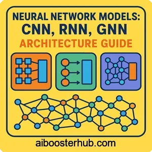
Neural Network Models: CNN, RNN, GNN Architecture Guide

Neural network architecture forms the backbone of modern artificial intelligence, powering everything from image recognition to natural language processing. Understanding different neural network models is essential for anyone working in deep learning, as each architecture solves specific types of problems with varying levels of efficiency. This comprehensive guide explores the most important neural network architectures, from foundational feedforward networks to cutting-edge transformer models, helping you choose the right approach for your AI projects.

Content

1. Understanding neural network architecture fundamentals

What makes up a neural network

At its core, a neural network model consists of interconnected layers of artificial neurons that process information. Each neural network layer in AI serves a specific purpose: the input layer receives data, hidden layers extract features and patterns, and the output layer produces predictions. The connections between neurons carry weights that adjust during training through backpropagation neural network algorithms.

The basic building block is the perceptron neural network, which takes multiple inputs, multiplies them by weights, adds a bias term, and passes the result through an activation function. Mathematically, a single neuron computes:

$$y = f\left(\sum_{i=1}^{n} w_i x_i + b\right)$$

where $w_i$ are weights, $x_i$ are inputs, $b$ is the bias, and $f$ is the activation function.

Key components across all architectures

Every neural network architecture shares common elements. The hidden layer sits between input and output, performing feature extraction and transformation. Activation functions like ReLU, sigmoid, or tanh introduce non-linearity, enabling networks to learn complex patterns. The backpropagation neural network training process computes gradients and updates weights to minimize prediction errors.

Deep neural networks contain multiple hidden layers, allowing hierarchical feature learning. Shallow networks with one or two layers work well for simple problems, but deep architectures excel at capturing intricate relationships in complex data.

2. Feedforward neural network: The foundation

How feed forward neural networks operate

The feedforward neural network represents the simplest neural network architecture where information flows in one direction—from input to output without loops. Also called a feed forward neural network or multilayer perceptron, this model processes data through sequential layers, with each layer fully connected to the next.

Here’s a simple Python implementation using PyTorch:

import torch
import torch.nn as nn

class FeedforwardNN(nn.Module):
    def __init__(self, input_size, hidden_size, output_size):
        super(FeedforwardNN, self).__init__()
        self.layer1 = nn.Linear(input_size, hidden_size)
        self.relu = nn.ReLU()
        self.layer2 = nn.Linear(hidden_size, output_size)
    
    def forward(self, x):
        x = self.layer1(x)
        x = self.relu(x)
        x = self.layer2(x)
        return x

# Example: 10 input features, 20 hidden neurons, 3 output classes
model = FeedforwardNN(10, 20, 3)
sample_input = torch.randn(1, 10)
output = model(sample_input)

Applications and limitations

Feedforward networks excel at classification and regression tasks with structured, tabular data. They’re commonly used for credit scoring, disease prediction, and simple pattern recognition. However, they struggle with sequential data since they lack memory of previous inputs, and they can’t handle variable-length inputs efficiently.

3. Convolutional neural networks: Vision specialists

Understanding CNN architecture

Convolutional neural networks revolutionized computer vision by introducing spatial awareness into neural network models. When people ask “what is CNN,” the answer lies in its unique architecture: convolutional layers that scan images with learnable filters, pooling layers that reduce dimensionality, and fully connected layers for final classification.

The convolutional operation applies a filter across the input, computing:

$$S(i,j) = (I * K)(i,j) = \sum_{m}\sum_{n} I(i+m, j+n)K(m,n)$$

where $I$ is the input image, $K$ is the filter kernel, and $*$ denotes convolution.

CNN in practice

Here’s a practical CNN implementation for image classification:

import torch.nn as nn

class SimpleCNN(nn.Module):
    def __init__(self, num_classes=10):
        super(SimpleCNN, self).__init__()
        # Convolutional layers
        self.conv1 = nn.Conv2d(3, 32, kernel_size=3, padding=1)
        self.conv2 = nn.Conv2d(32, 64, kernel_size=3, padding=1)
        self.pool = nn.MaxPool2d(2, 2)
        
        # Fully connected layers
        self.fc1 = nn.Linear(64 * 8 * 8, 128)
        self.fc2 = nn.Linear(128, num_classes)
        self.relu = nn.ReLU()
        self.dropout = nn.Dropout(0.5)
    
    def forward(self, x):
        x = self.pool(self.relu(self.conv1(x)))
        x = self.pool(self.relu(self.conv2(x)))
        x = x.view(-1, 64 * 8 * 8)
        x = self.relu(self.fc1(x))
        x = self.dropout(x)
        x = self.fc2(x)
        return x

CNN models dominate image classification, object detection, facial recognition, and medical image analysis. Popular architectures like ResNet, VGG, and EfficientNet have achieved human-level performance on various vision tasks.

4. Recurrent neural network: Handling sequences

The power of memory in RNNs

The recurrent neural network introduces temporal dynamics to neural network architecture by maintaining an internal state or “memory.” Unlike feedforward networks, recurrent neural networks process sequential data by feeding outputs back into the network, allowing them to capture temporal dependencies.

The basic RNN update equation is:

$$h_t = f(W_{hh}h_{t-1} + W_{xh}x_t + b_h)$$

$$y_t = W_{hy}h_t + b_y$$

where $h_t$ is the hidden state at time $t$, $x_t$ is the input, and $W$ matrices are learnable weights.

LSTM neural network: Solving the gradient problem

Standard RNNs struggle with long-term dependencies due to vanishing gradients. The LSTM neural network architecture addresses this with gating mechanisms that control information flow:

import torch.nn as nn

class LSTMModel(nn.Module):
    def __init__(self, input_size, hidden_size, num_layers, output_size):
        super(LSTMModel, self).__init__()
        self.hidden_size = hidden_size
        self.num_layers = num_layers
        
        self.lstm = nn.LSTM(input_size, hidden_size, num_layers, 
                           batch_first=True)
        self.fc = nn.Linear(hidden_size, output_size)
    
    def forward(self, x):
        # Initialize hidden and cell states
        h0 = torch.zeros(self.num_layers, x.size(0), self.hidden_size)
        c0 = torch.zeros(self.num_layers, x.size(0), self.hidden_size)
        
        # LSTM forward pass
        out, _ = self.lstm(x, (h0, c0))
        
        # Get last time step output
        out = self.fc(out[:, -1, :])
        return out

# Example: sequence classification
model = LSTMModel(input_size=50, hidden_size=128, 
                  num_layers=2, output_size=5)

LSTM and GRU (Gated Recurrent Unit) variants excel at language modeling, machine translation, speech recognition, and time series forecasting.

5. Graph neural network: Learning from relationships

What is GNN and why it matters

Graph neural networks represent a paradigm shift in neural network models, designed specifically for graph-structured data where relationships between entities matter as much as the entities themselves. A GNN learns representations by aggregating information from neighboring nodes, making them ideal for social networks, molecular structures, and knowledge graphs.

The message-passing framework in GNNs can be expressed as:

$$h_v^{(k+1)} = \text{UPDATE}^{(k)}\left(h_v^{(k)}, \text{AGGREGATE}^{(k)}\left({h_u^{(k)} : u \in \mathcal{N}(v)}\right)\right)$$

where $h_v^{(k)}$ is the node representation at layer $k$, and $\mathcal{N}(v)$ represents neighbors of node $v$.

Implementing a basic GNN

Here’s a simple graph convolutional network implementation:

import torch
import torch.nn as nn
import torch.nn.functional as F

class GCNLayer(nn.Module):
    def __init__(self, in_features, out_features):
        super(GCNLayer, self).__init__()
        self.linear = nn.Linear(in_features, out_features)
    
    def forward(self, x, adjacency_matrix):
        # Aggregate neighbor features
        support = self.linear(x)
        output = torch.matmul(adjacency_matrix, support)
        return output

class GNN(nn.Module):
    def __init__(self, input_dim, hidden_dim, output_dim):
        super(GNN, self).__init__()
        self.gcn1 = GCNLayer(input_dim, hidden_dim)
        self.gcn2 = GCNLayer(hidden_dim, output_dim)
    
    def forward(self, x, adj):
        x = F.relu(self.gcn1(x, adj))
        x = self.gcn2(x, adj)
        return x

# Example usage
model = GNN(input_dim=16, hidden_dim=32, output_dim=8)

Graph neural networks power recommendation systems, drug discovery, traffic prediction, and social network analysis. Popular GNN architectures include Graph Convolutional Networks (GCN), GraphSAGE, and Graph Attention Networks (GAT).

6. Advanced neural network architectures

Transformer neural network: The attention revolution

The transformer neural network architecture revolutionized deep learning by replacing recurrence with self-attention mechanisms. This parallel processing capability makes transformers significantly faster than recurrent neural networks while capturing long-range dependencies more effectively.

The core self-attention mechanism computes:

$$\text{Attention}(Q, K, V) = \text{softmax}\left(\frac{QK^T}{\sqrt{d_k}}\right)V$$

where $Q$ (query), $K$ (key), and $V$ (value) are learned linear projections of the input.

Transformers dominate natural language processing tasks, powering models like GPT, BERT, and T5. They’ve also expanded into computer vision with Vision Transformers (ViT).

Specialized architectures for unique challenges

Bayesian neural network models incorporate uncertainty quantification by treating weights as probability distributions rather than fixed values. This makes them valuable for risk-sensitive applications like medical diagnosis and autonomous driving.

Siamese neural network architectures use twin networks with shared weights to learn similarity metrics. They excel at one-shot learning, face verification, and signature verification by comparing pairs of inputs.

Spiking neural network (SNNs) models mimic biological neurons more closely by communicating through discrete spikes rather than continuous values. These energy-efficient networks show promise for neuromorphic computing and edge AI devices.

Liquid neural networks represent cutting-edge research with time-continuous models that adapt their behavior dynamically. These flexible architectures can adjust to new data distributions without retraining, making them suitable for robotics and autonomous systems.

Comparing neural network models

Different nn models suit different tasks:

Feedforward networks: Structured tabular data, simple classification
CNNs: Image processing, spatial pattern recognition
RNNs/LSTMs: Sequential data, time series, natural language
GNNs: Graph-structured data, relational reasoning
Transformers: Long-range dependencies, parallel processing needs
Specialized networks: Domain-specific requirements

7. Choosing and implementing the right architecture

Selection criteria for neural network models

Selecting the appropriate neural network architecture depends on several factors. Consider your data structure first: images suggest CNNs, sequences point to RNNs or transformers, and graphs require GNNs. Computational resources matter—transformers demand significant memory and processing power, while simpler feedforward networks run efficiently on limited hardware.

Task complexity influences depth and width. Deep neural networks with many layers capture intricate patterns but require more training data and computational resources. Start with simpler architectures and increase complexity only when necessary to avoid overfitting.

Best practices for training neural network models

Effective training requires proper initialization, learning rate scheduling, and regularization. Batch normalization stabilizes training in deep networks, while dropout prevents overfitting. Data augmentation artificially expands training sets, particularly valuable for CNNs in computer vision tasks.

Monitor validation metrics to detect overfitting early. Use techniques like early stopping, weight decay, and cross-validation to ensure your neural network model generalizes well to unseen data. Experiment with different optimizers—Adam works well for most cases, but SGD with momentum can achieve better final performance with careful tuning.

Hybrid approaches and ensemble methods

Modern deep learning often combines multiple neural network architectures. CNN-LSTM hybrids process video data by using convolutional layers for spatial features and recurrent layers for temporal dynamics. Transformer-CNN combinations capture both local patterns and global context in images.

Ensemble methods that combine predictions from multiple models often outperform single architectures. Training several neural network models with different initializations or architectures and averaging their predictions reduces variance and improves robustness.

8. Knowledge Check

Quiz 1: Core Network Layers

Question: What are the three primary types of layers in a neural network and what is the specific purpose of each?

Answer: The three primary layers are:

• Input Layer: Receives the initial raw data for the network to process.

• Hidden Layers: Perform non-linear transformations to extract features and learn complex patterns from the data.

• Output Layer: Produces the final prediction, classification, or other desired result.

Quiz 2: Feedforward Network Limitations

Question: What is a key limitation of Feedforward Neural Networks when dealing with certain types of data?

Answer: Their core limitation is an inability to handle sequential data. Because information flows in only one direction, they have no memory of previous inputs, a weakness that prompted the development of more advanced, sequence-aware architectures.

Quiz 3: The Vision Specialists

Question: Which neural network architecture revolutionized computer vision, and what core architectural feature gives it this capability?

Answer: Convolutional Neural Networks (CNNs) revolutionized computer vision by introducing spatial awareness. They achieve this through the use of convolutional layers, which scan images with learnable filters to detect hierarchies of features like edges, shapes, and objects.

Quiz 4: The Power of Memory

Question: What fundamental feature allows Recurrent Neural Networks (RNNs) to process sequential data effectively?

Answer: Addressing the key limitation of feedforward networks, Recurrent Neural Networks (RNNs) maintain an internal state, or “memory.” They accomplish this by feeding outputs from a previous step back into the network as an input for the current step, allowing them to capture temporal dependencies in data like text or time series.

Quiz 5: Solving the Gradient Problem

Question: What significant problem in standard RNNs is addressed by the Long Short-Term Memory (LSTM) architecture?

Answer: LSTMs solve the critical problem of vanishing gradients, which prevents standard RNNs from effectively learning long-term dependencies in a sequence. They achieve this using sophisticated gating mechanisms (e.g., forget, input, and output gates that regulate the flow of information through the cell’s memory), allowing the network to retain important information over long periods.

Quiz 6: Learning from Relationships

Question: For what specific type of data are Graph Neural Networks (GNNs) primarily designed?

Answer: Graph Neural Networks (GNNs) are specifically designed for graph-structured data, where the relationships between entities are as important as the entities themselves. This makes them ideal for analyzing social networks, molecular structures, and knowledge graphs.

Quiz 7: The Attention Revolution

Question: What core mechanism allows the Transformer architecture to process data in parallel and capture long-range dependencies more effectively than RNNs?

Answer: As a powerful successor to the recurrent approach, the Transformer architecture replaced loops with self-attention mechanisms, which allow the model to weigh the importance of different words in an input sequence simultaneously. This innovation enables massive parallel processing and is more effective at capturing long-range dependencies, powering flagship models like GPT, BERT, and T5.

Quiz 8: Learning Similarity

Question: What is the main purpose of a Siamese neural network?

Answer: A Siamese network is designed to learn a similarity metric between two inputs. It uses twin networks with shared weights to process two distinct inputs and determine how similar they are, making it ideal for tasks like face verification and signature verification.

Quiz 9: Biologically-Inspired Computing

Question: How does a Spiking Neural Network (SNN) mimic biological neurons in its method of communication?

Answer: Spiking Neural Networks (SNNs) more closely mimic biological neurons by communicating through discrete spikes fired over time, rather than the continuous values used in most other architectures. This event-driven approach makes them highly energy-efficient and promising for neuromorphic computing.

Quiz 10: The First Step in Model Selection

Question: According to the guide, what is the first and most important factor to consider when choosing the right neural network architecture for a project?

Answer: The first and most critical factor is the data structure. The nature of your data provides the clearest starting point for model selection: images suggest CNNs, sequences point to RNNs or Transformers, and interconnected graphs require GNNs.

Explore more: