Neural Networks Explained: From Basics to Practice

Artificial intelligence has transformed from science fiction into everyday reality, powering everything from smartphone assistants to medical diagnosis systems. At the heart of this revolution lies a fascinating technology inspired by the human brain: neural networks. If you’ve ever wondered how machines learn to recognize faces, translate languages, or drive cars, you’re about to discover the answer.

This comprehensive guide will demystify neural networks, breaking down complex concepts into digestible explanations with practical examples. Whether you’re a student, developer, or simply curious about AI, you’ll gain a solid understanding of what neural networks are, how they work, and why they’ve become indispensable in modern technology.

1. What is a neural network?

A neural network is a computational model inspired by the way biological neurons in the human brain process information. At its core, a neural network is a system of interconnected nodes (called neurons or units) that work together to recognize patterns, make decisions, and learn from data.

Neural network definition

The neural network definition encompasses several key characteristics: it’s a machine learning model composed of layers of artificial neurons that can learn complex patterns through training. Each connection between neurons has an associated weight that adjusts during learning, allowing the network to improve its performance over time.

Think of a neural network as a sophisticated pattern recognition machine. Just as your brain learns to recognize your friend’s face through repeated exposure, a neural network learns to identify patterns in data by processing thousands or millions of examples. The neural meaning extends beyond simple computation—it represents a fundamental shift in how we approach problem-solving with computers.

ANN model fundamentals

An ANN model (Artificial Neural Network model) consists of three essential components:

Input Layer: This is where data enters the network. Each neuron in the input layer represents a feature of your data. For example, in an image recognition task, each pixel might correspond to an input neuron.

Hidden Layers: These intermediate layers perform the computational heavy lifting. The term “hidden” simply means they’re not directly observable from the input or output. This is where the neural computation and pattern extraction happen.

Output Layer: This produces the network’s final prediction or classification. For a cat-versus-dog classifier, you might have two output neurons representing the probability of each class.

The connections between these layers form what we call the neural network architecture. Each connection carries information forward through the network in a process called forward propagation.

2. The history and discovery of neural networks

Understanding who discovered neural networks requires looking at several pioneering contributions that shaped this field.

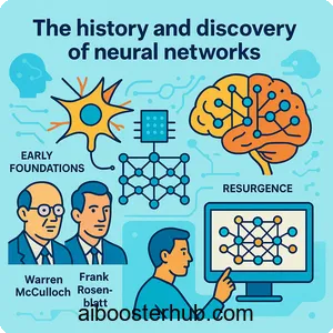
Early foundations

The neural concept originated in the 1940s when Warren McCulloch and Walter Pitts created the first mathematical model of an artificial neuron. Their groundbreaking paper demonstrated that simple artificial neurons could, in theory, compute any arithmetic or logical function.

Frank Rosenblatt advanced this work significantly by inventing the Perceptron in the late 1950s—the first neural network implementation that could actually learn. The Perceptron was a single-layer neural network that could classify simple patterns. Rosenblatt famously demonstrated his invention by teaching it to recognize letters and shapes.

The AI winters and resurgence

The field experienced dramatic ups and downs. In the 1960s, researchers discovered that simple perceptrons couldn’t solve certain problems, leading to reduced funding and interest—a period known as the “AI winter.” However, the development of backpropagation algorithms in the 1980s breathed new life into neural network research, enabling multi-layer networks to learn complex patterns.

The modern renaissance began when increased computational power and massive datasets made deep learning practical. This convergence of factors transformed neural networks from academic curiosities into powerful tools that outperform traditional methods in many domains.

3. How neural networks work

To truly understand neural network AI, we need to explore the mechanics of how these systems process information and learn.

The artificial neuron

Each neuron performs a simple operation: it receives inputs, multiplies them by weights, adds a bias term, and passes the result through an activation function. Mathematically, a single neuron computes:

$$z = w_1x_1 + w_2x_2 + … + w_nx_n + b$$

$$a = f(z)$$

Where:

• \(x_i\) are the inputs
• \(w_i\) are the weights
• \(b\) is the bias
• \(f\) is the activation function
• \(a\) is the neuron’s output

The activation function introduces non-linearity, allowing the network to learn complex patterns. Common activation functions include ReLU (Rectified Linear Unit), sigmoid, and tanh.

Forward propagation

During forward propagation, data flows from the input layer through the hidden layers to the output layer. Each layer transforms the data, extracting increasingly abstract features. In image recognition, early layers might detect edges, middle layers might identify shapes, and deeper layers might recognize entire objects.

Here’s a simple Python implementation showing forward propagation through a single layer:

import numpy as np

def sigmoid(x):
    """Sigmoid activation function"""
    return 1 / (1 + np.exp(-x))

def forward_propagation(X, weights, bias):
    """
    Perform forward propagation through one layer
    
    Args:
        X: Input data (n_samples, n_features)
        weights: Weight matrix (n_features, n_neurons)
        bias: Bias vector (n_neurons,)
    
    Returns:
        Activation output
    """
    # Linear transformation
    z = np.dot(X, weights) + bias
    
    # Apply activation function
    a = sigmoid(z)
    
    return a

# Example usage
X = np.array([[0.5, 0.3, 0.2]])  # Single input sample
weights = np.array([[0.4, 0.7],
                    [0.3, 0.5],
                    [0.6, 0.2]])  # 3 inputs to 2 neurons
bias = np.array([0.1, 0.2])

output = forward_propagation(X, weights, bias)
print(f"Layer output: {output}")

Backpropagation and learning

The magic of neural networks lies in their ability to learn. This happens through backpropagation—an algorithm that adjusts weights to minimize prediction errors. The process works like this:

1. Make a prediction: Run forward propagation with current weights
2. Calculate error: Compare prediction to actual target using a loss function
3. Compute gradients: Determine how much each weight contributed to the error
4. Update weights: Adjust weights in the direction that reduces error

The loss function quantifies how wrong the network’s predictions are. For example, Mean Squared Error (MSE) is commonly used for regression problems:

$$L = \frac{1}{n}\sum_{i=1}^{n}(y_i – \hat{y}_i)^2$$

Where \(y_i\) is the true value and \(\hat{y}_i\) is the predicted value.

Weights are updated using gradient descent:

$$w_{new} = w_{old} – \alpha \frac{\partial L}{\partial w}$$

Where \(\alpha\) is the learning rate, controlling how large the weight updates are.

Here’s a complete example of training a simple neural network:

import numpy as np

class SimpleNeuralNetwork:
    def __init__(self, input_size, hidden_size, output_size, learning_rate=0.1):
        """Initialize a simple 2-layer neural network"""
        # Initialize weights randomly
        self.W1 = np.random.randn(input_size, hidden_size) * 0.01
        self.b1 = np.zeros((1, hidden_size))
        self.W2 = np.random.randn(hidden_size, output_size) * 0.01
        self.b2 = np.zeros((1, output_size))
        self.learning_rate = learning_rate
    
    def sigmoid(self, x):
        """Sigmoid activation function"""
        return 1 / (1 + np.exp(-np.clip(x, -500, 500)))
    
    def sigmoid_derivative(self, x):
        """Derivative of sigmoid function"""
        return x * (1 - x)
    
    def forward(self, X):
        """Forward propagation"""
        self.z1 = np.dot(X, self.W1) + self.b1
        self.a1 = self.sigmoid(self.z1)
        self.z2 = np.dot(self.a1, self.W2) + self.b2
        self.a2 = self.sigmoid(self.z2)
        return self.a2
    
    def backward(self, X, y, output):
        """Backpropagation"""
        m = X.shape[0]
        
        # Calculate gradients
        dz2 = output - y
        dW2 = np.dot(self.a1.T, dz2) / m
        db2 = np.sum(dz2, axis=0, keepdims=True) / m
        
        dz1 = np.dot(dz2, self.W2.T) * self.sigmoid_derivative(self.a1)
        dW1 = np.dot(X.T, dz1) / m
        db1 = np.sum(dz1, axis=0, keepdims=True) / m
        
        # Update weights
        self.W2 -= self.learning_rate * dW2
        self.b2 -= self.learning_rate * db2
        self.W1 -= self.learning_rate * dW1
        self.b1 -= self.learning_rate * db1
    
    def train(self, X, y, epochs):
        """Train the neural network"""
        losses = []
        for epoch in range(epochs):
            # Forward propagation
            output = self.forward(X)
            
            # Calculate loss
            loss = np.mean((y - output) ** 2)
            losses.append(loss)
            
            # Backpropagation
            self.backward(X, y, output)
            
            if epoch % 100 == 0:
                print(f"Epoch {epoch}, Loss: {loss:.4f}")
        
        return losses

# Example: XOR problem
X = np.array([[0, 0], [0, 1], [1, 0], [1, 1]])
y = np.array([[0], [1], [1], [0]])

# Create and train network
nn = SimpleNeuralNetwork(input_size=2, hidden_size=4, output_size=1, learning_rate=0.5)
losses = nn.train(X, y, epochs=1000)

# Test predictions
predictions = nn.forward(X)
print("\nFinal Predictions:")
for i in range(len(X)):
    print(f"Input: {X[i]} -> Predicted: {predictions[i][0]:.4f}, Actual: {y[i][0]}")

4. Types of neural network architectures

Neural networks come in various architectures, each designed for specific types of problems. Understanding these different neural net designs helps you choose the right tool for your task.

Feedforward neural networks

The simplest type, where information flows in one direction from input to output without loops. These are ideal for classification and regression problems with structured data. A multi-layer perceptron (MLP) is a common example, featuring fully connected layers where each neuron connects to all neurons in the next layer.

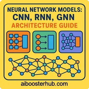
Convolutional neural networks (CNNs)

CNNs excel at processing grid-like data such as images. They use specialized layers called convolutional layers that scan across the input, detecting local patterns like edges and textures. This neural network visualization concept is crucial—CNNs preserve spatial relationships in data, making them perfect for computer vision tasks.

A typical CNN architecture includes:

• Convolutional layers: Extract features through learnable filters
• Pooling layers: Reduce spatial dimensions while retaining important information
• Fully connected layers: Make final classifications based on extracted features

Recurrent neural networks (RNNs)

RNNs are designed for sequential data like text, speech, or time series. Unlike feedforward networks, RNNs have connections that loop back, allowing them to maintain a “memory” of previous inputs. This makes them ideal for tasks where context matters, such as language translation or speech recognition.

Advanced RNN variants like LSTM (Long Short-Term Memory) and GRU (Gated Recurrent Unit) address the challenge of learning long-term dependencies.

Transformer networks

Transformers have revolutionized natural language processing and beyond. They use attention mechanisms to weigh the importance of different parts of the input, allowing them to capture relationships across long sequences efficiently. These form the backbone of modern language models.

5. Practical applications of neural networks

Neural networks have moved from research labs into countless real-world applications, fundamentally changing how we interact with technology.

Computer vision

Neural networks power image recognition systems that can identify objects, faces, and scenes with remarkable accuracy. Applications include:

• Medical imaging: Detecting tumors, fractures, and diseases from X-rays, MRIs, and CT scans
• Autonomous vehicles: Recognizing pedestrians, traffic signs, and road conditions
• Security systems: Facial recognition for authentication and surveillance
• Quality control: Identifying defects in manufacturing processes

Natural language processing

Understanding and generating human language is where neural networks truly shine:

• Machine translation: Real-time translation between languages
• Sentiment analysis: Understanding emotions and opinions in text
• Chatbots and virtual assistants: Conversational AI that understands context
• Text generation: Creating human-like written content

Speech and audio processing

Neural networks can both understand and generate speech:

• Voice assistants: Converting speech to text and responding intelligently
• Music generation: Creating original compositions in various styles
• Audio enhancement: Removing noise and improving sound quality

Recommendation systems

Every time you see personalized content suggestions, neural networks are working behind the scenes:

• Streaming services: Recommending movies, shows, and music
• E-commerce: Suggesting products based on browsing and purchase history
• Social media: Curating your feed based on interests and engagement

Game playing and robotics

Neural networks enable machines to master complex tasks:

• Game AI: Systems that can defeat human champions in chess, Go, and video games
• Robot control: Enabling robots to navigate environments and manipulate objects
• Industrial automation: Optimizing manufacturing processes and logistics

6. Building your first neural network

Let’s create a practical neural network for a real classification problem: recognizing handwritten digits. This example uses a popular dataset and demonstrates the complete workflow.

import numpy as np
from sklearn.datasets import load_digits
from sklearn.model_selection import train_test_split
from sklearn.preprocessing import StandardScaler
import matplotlib.pyplot as plt

class DigitClassifier:
    def __init__(self, layer_sizes, learning_rate=0.01):
        """
        Initialize neural network for digit classification
        
        Args:
            layer_sizes: List of layer sizes [input, hidden1, hidden2, ..., output]
            learning_rate: Learning rate for gradient descent
        """
        self.layer_sizes = layer_sizes
        self.learning_rate = learning_rate
        self.weights = []
        self.biases = []
        
        # Initialize weights and biases for each layer
        for i in range(len(layer_sizes) - 1):
            w = np.random.randn(layer_sizes[i], layer_sizes[i+1]) * 0.01
            b = np.zeros((1, layer_sizes[i+1]))
            self.weights.append(w)
            self.biases.append(b)
    
    def relu(self, x):
        """ReLU activation function"""
        return np.maximum(0, x)
    
    def relu_derivative(self, x):
        """Derivative of ReLU"""
        return (x > 0).astype(float)
    
    def softmax(self, x):
        """Softmax activation for output layer"""
        exp_x = np.exp(x - np.max(x, axis=1, keepdims=True))
        return exp_x / np.sum(exp_x, axis=1, keepdims=True)
    
    def forward_propagation(self, X):
        """Forward pass through the network"""
        self.activations = [X]
        self.z_values = []
        
        # Forward through hidden layers
        for i in range(len(self.weights) - 1):
            z = np.dot(self.activations[-1], self.weights[i]) + self.biases[i]
            self.z_values.append(z)
            a = self.relu(z)
            self.activations.append(a)
        
        # Output layer with softmax
        z = np.dot(self.activations[-1], self.weights[-1]) + self.biases[-1]
        self.z_values.append(z)
        a = self.softmax(z)
        self.activations.append(a)
        
        return self.activations[-1]
    
    def compute_loss(self, y_true, y_pred):
        """Compute cross-entropy loss"""
        m = y_true.shape[0]
        log_likelihood = -np.log(y_pred[range(m), y_true])
        loss = np.sum(log_likelihood) / m
        return loss
    
    def backward_propagation(self, X, y):
        """Backward pass - compute gradients"""
        m = X.shape[0]
        
        # Convert y to one-hot encoding
        y_one_hot = np.zeros((m, self.layer_sizes[-1]))
        y_one_hot[range(m), y] = 1
        
        # Output layer gradient
        dz = self.activations[-1] - y_one_hot
        gradients_w = []
        gradients_b = []
        
        # Backpropagate through layers
        for i in range(len(self.weights) - 1, -1, -1):
            dw = np.dot(self.activations[i].T, dz) / m
            db = np.sum(dz, axis=0, keepdims=True) / m
            gradients_w.insert(0, dw)
            gradients_b.insert(0, db)
            
            if i > 0:
                dz = np.dot(dz, self.weights[i].T) * self.relu_derivative(self.z_values[i-1])
        
        return gradients_w, gradients_b
    
    def update_parameters(self, gradients_w, gradients_b):
        """Update weights and biases using gradients"""
        for i in range(len(self.weights)):
            self.weights[i] -= self.learning_rate * gradients_w[i]
            self.biases[i] -= self.learning_rate * gradients_b[i]
    
    def train(self, X_train, y_train, X_val, y_val, epochs=100):
        """Train the neural network"""
        train_losses = []
        val_accuracies = []
        
        for epoch in range(epochs):
            # Forward propagation
            y_pred = self.forward_propagation(X_train)
            
            # Compute loss
            loss = self.compute_loss(y_train, y_pred)
            train_losses.append(loss)
            
            # Backward propagation
            gradients_w, gradients_b = self.backward_propagation(X_train, y_train)
            
            # Update parameters
            self.update_parameters(gradients_w, gradients_b)
            
            # Validation accuracy
            val_acc = self.evaluate(X_val, y_val)
            val_accuracies.append(val_acc)
            
            if epoch % 10 == 0:
                print(f"Epoch {epoch}: Loss = {loss:.4f}, Val Accuracy = {val_acc:.4f}")
        
        return train_losses, val_accuracies
    
    def predict(self, X):
        """Make predictions"""
        y_pred = self.forward_propagation(X)
        return np.argmax(y_pred, axis=1)
    
    def evaluate(self, X, y):
        """Evaluate accuracy"""
        predictions = self.predict(X)
        accuracy = np.mean(predictions == y)
        return accuracy

# Load and prepare data
digits = load_digits()
X, y = digits.data, digits.target

# Split data
X_train, X_test, y_train, y_test = train_test_split(X, y, test_size=0.2, random_state=42)

# Normalize features
scaler = StandardScaler()
X_train = scaler.fit_transform(X_train)
X_test = scaler.transform(X_test)

# Create and train neural network
nn = DigitClassifier(layer_sizes=[64, 32, 16, 10], learning_rate=0.1)
train_losses, val_accuracies = nn.train(X_train, y_train, X_test, y_test, epochs=100)

# Final evaluation
final_accuracy = nn.evaluate(X_test, y_test)
print(f"\nFinal Test Accuracy: {final_accuracy:.4f}")

# Visualize some predictions
predictions = nn.predict(X_test[:10])
print("\nSample Predictions:")
for i in range(10):
    print(f"Predicted: {predictions[i]}, Actual: {y_test[i]}")

Understanding the code

This implementation demonstrates how is neural networks made in practice:

1. Architecture design: We define layer sizes, creating a network with 64 input neurons (for 8×8 pixel images), two hidden layers, and 10 output neurons (for digits 0-9)
2. Activation functions: ReLU for hidden layers provides non-linearity while avoiding vanishing gradients. Softmax in the output layer produces probability distributions
3. Loss function: Cross-entropy loss is ideal for classification tasks, penalizing confident wrong predictions more heavily
4. Training loop: Each epoch involves forward propagation, loss calculation, backpropagation, and parameter updates

This nn model achieves strong performance on digit recognition, typically reaching over 95% accuracy with proper tuning.

7. Challenges and best practices

While neural networks are powerful, building effective models requires understanding common pitfalls and solutions.

Overfitting and underfitting

Overfitting occurs when your network memorizes training data rather than learning generalizable patterns. Signs include high training accuracy but poor test performance. Solutions include:

• Regularization: Add penalties for large weights (L1 or L2 regularization)
• Dropout: Randomly deactivate neurons during training to prevent co-adaptation
• Early stopping: Stop training when validation performance plateaus
• Data augmentation: Create variations of training examples

Underfitting happens when the network is too simple to capture patterns in the data. Address this by:

• Increasing network complexity (more layers or neurons)
• Training for more epochs
• Reducing regularization strength
• Adding relevant features

Choosing hyperparameters

Critical hyperparameters include:

• Learning rate: Too high causes instability; too low means slow convergence. Start with values between 0.001 and 0.1
• Batch size: Larger batches provide stable gradients but require more memory. Typical values: 32, 64, 128
• Network architecture: Start simple and add complexity as needed
• Number of epochs: Train until validation performance stops improving

Data preparation

Quality data is fundamental to neural network success:

• Normalization: Scale features to similar ranges (typically 0-1 or standardized)
• Handling missing values: Impute or remove incomplete samples
• Balancing classes: Ensure training data represents all classes adequately
• Train-validation-test split: Maintain separate datasets to evaluate generalization

Computational considerations

Where is neural networks found in terms of computational resources? Training neural networks demands significant computing power:

• GPU acceleration: Essential for deep networks and large datasets
• Batch processing: Process multiple samples simultaneously for efficiency
• Model compression: Techniques like pruning and quantization reduce model size for deployment

Debugging neural networks

When your neural network isn’t learning:

1. Check data pipeline: Verify inputs are correctly preprocessed and labels are accurate
2. Start simple: Begin with a small network and gradually increase complexity
3. Monitor gradients: Vanishing or exploding gradients indicate architectural issues
4. Visualize learning curves: Plot training and validation loss to diagnose problems
5. Test components individually: Verify each layer and function works as expected

8. Conclusion

Neural networks represent one of humanity’s most remarkable technological achievements—computational systems that learn from experience, recognize patterns, and solve problems that once seemed impossible for machines. From their biological inspiration to their mathematical foundations, we’ve explored what is a neural network at multiple levels of understanding.

The journey from simple perceptrons to today’s sophisticated deep learning systems showcases the power of persistent research and innovation. Whether you’re building your first neural network or exploring advanced architectures, remember that these systems are tools designed to augment human intelligence, not replace it. As you continue learning about neural network AI, you’ll discover endless opportunities to apply these techniques to real-world problems. The field continues to evolve rapidly, offering exciting possibilities for those willing to dive deeper into this transformative technology.