Neural Radiance Fields (NeRF): 3D Scene Representation

The ability to capture and reconstruct three-dimensional scenes from two-dimensional images has long been a cornerstone challenge in computer vision and graphics. Traditional methods have relied on explicit representations like point clouds, meshes, or voxel grids, each with their own limitations in terms of memory efficiency, rendering quality, or geometric flexibility. However, neural radiance fields (NeRF) represent a paradigm shift in how we approach 3D scene representation, leveraging the power of neural networks to encode complex scenes as continuous functions. Moreover, this breakthrough in neural rendering has opened new possibilities for view synthesis, 3D reconstruction, and immersive content creation.

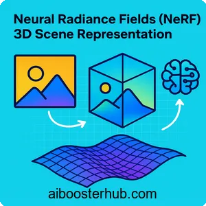
At its core, NeRF uses implicit neural representation to model how light interacts with a scene. Specifically, by training a neural network to map 3D coordinates and viewing directions to color and density values, NeRF can synthesize photorealistic novel views of scenes with unprecedented quality. As a result, this approach has revolutionized applications ranging from virtual reality and augmented reality to film production and cultural heritage preservation.

Content

1. Understanding neural radiance fields

What are neural radiance fields?

Neural radiance fields represent a fundamentally different approach to 3D scene representation. Instead of storing geometric information explicitly, NeRF encodes a scene as a continuous 5D function that maps any 3D location $ \mathbf{x} = (x, y, z) $ and viewing direction $ \mathbf{d} = (\theta, \phi) $ to a volume density $ \sigma $ and emitted color $ \mathbf{c} = (r, g, b) $.

The core idea is that every point in 3D space can be queried to determine its opacity (density) and the color of light emitted in a particular direction. Consequently, this allows NeRF to model view-dependent effects like specular reflections and translucency naturally. Furthermore, the function is represented by a multilayer perceptron (MLP), a type of neural network, which learns to predict these values through training on a set of images with known camera poses.

The mathematical foundation

The NeRF function can be expressed as:

$$ F_{\Theta}: (\mathbf{x}, \mathbf{d}) \rightarrow (\mathbf{c}, \sigma) $$

where $ \Theta $ represents the network parameters. To render a pixel in a novel view, NeRF uses volumetric rendering. A camera ray $ \mathbf{r}(t) = \mathbf{o} + t\mathbf{d} $ is cast through the scene, where $ \mathbf{o} $ is the camera origin and $ \mathbf{d} $ is the ray direction.

The expected color $ C(\mathbf{r}) $ along this ray is computed by integrating the contribution of all points:

$$ C(\mathbf{r}) = \int_{t_n}^{t_f} T(t) \sigma(\mathbf{r}(t)) \mathbf{c}(\mathbf{r}(t), \mathbf{d}) dt $$

where $ T(t) $ is the accumulated transmittance:

$$ T(t) = \exp\left(-\int_{t_n}^{t} \sigma(\mathbf{r}(s)) ds\right) $$

This transmittance represents the probability that a ray travels from $ t_n $ to $ t $ without hitting any particles. In practice, this continuous integral is approximated using numerical quadrature with stratified sampling along the ray.

Why implicit neural representations matter

The shift to implicit neural representation offers several key advantages over traditional explicit methods:

Memory efficiency: Instead of storing millions of vertices or voxels, NeRF stores scene information in the weights of a relatively compact neural network. For instance, a typical NeRF model might use only 5-10 MB to represent a complex scene that would require gigabytes in voxel form.

Continuous representation: Unlike discrete representations, NeRF can be queried at arbitrary resolutions. Therefore, this means you can render the scene at any level of detail without being limited by the original sampling resolution.

Natural handling of complex geometry: Moreover, NeRF excels at representing intricate structures like hair, foliage, or semi-transparent materials that are challenging for traditional mesh-based approaches.

2. The NeRF architecture and training process

Network architecture

The NeRF neural network typically consists of a deep MLP with skip connections. The architecture processes the input in two stages:

Position encoding: The 3D coordinate $ \mathbf{x} $ is fed through 8 fully connected layers (with ReLU activations and 256 channels) to predict the volume density $ \sigma $ and a 256-dimensional feature vector.
Direction encoding: This feature vector is concatenated with the viewing direction $ \mathbf{d} $ and passed through one additional fully connected layer to produce the RGB color $ \mathbf{c} $.

A critical component is positional encoding, which applies high-frequency functions to the inputs before feeding them to the network:

$$ \gamma(p) = \left(\sin(2^0 \pi p), \cos(2^0 \pi p), \ldots, \sin(2^{L-1} \pi p), \cos(2^{L-1} \pi p)\right) $$

This encoding helps the network learn high-frequency details in both geometry and color. Without it, neural networks tend to bias toward learning lower frequency functions.

Training procedure

Training a NeRF model requires a dataset of images with known camera poses. The process follows these steps:

Data preparation: First, collect multiple images of the scene from different viewpoints with calibrated camera parameters (intrinsics and extrinsics).
Ray generation: Next, for each training image, generate camera rays for a batch of pixels.
Point sampling: Then, sample points along each ray using stratified sampling to ensure coverage across the entire ray.
Network evaluation: After that, query the neural network at each sampled point to obtain density and color values.
Volume rendering: Subsequently, compute the predicted color for each ray using the volumetric rendering equation.
Loss computation: Finally, calculate the mean squared error between predicted and ground truth pixel colors.

The optimization objective is:

$$ \mathcal{L} = \sum_{\mathbf{r} \in \mathcal{R}} \left| C(\mathbf{r}) – \hat{C}(\mathbf{r}) \right|_2^2 $$

where $ \mathcal{R} $ is the set of rays in the batch, $ C(\mathbf{r}) $ is the predicted color, and $ \hat{C}(\mathbf{r}) $ is the ground truth color.

Hierarchical volume sampling

Standard NeRF uses a hierarchical sampling strategy to improve efficiency. Specifically, it trains two networks simultaneously:

A coarse network that samples points uniformly along rays
A fine network that samples more densely near surfaces where the volume density is high

As a result, this approach allocates more computational resources to regions that contribute most to the final rendering, significantly improving both quality and efficiency.

3. Implementing NeRF in Python

Let’s walk through a simplified implementation of key NeRF components using Python and PyTorch. In this section, we’ll build the core functionality step by step:

import torch
import torch.nn as nn
import numpy as np

class PositionalEncoder(nn.Module):
    """Applies positional encoding to input coordinates."""
    
    def __init__(self, num_freqs=10, include_input=True):
        super().__init__()
        self.num_freqs = num_freqs
        self.include_input = include_input
        self.freq_bands = 2.0 ** torch.linspace(0, num_freqs - 1, num_freqs)
        
    def forward(self, x):
        """
        Args:
            x: Input tensor of shape [..., C]
        Returns:
            Encoded tensor of shape [..., C * (2 * num_freqs + 1)]
        """
        encoded = []
        if self.include_input:
            encoded.append(x)
            
        for freq in self.freq_bands:
            encoded.append(torch.sin(freq * np.pi * x))
            encoded.append(torch.cos(freq * np.pi * x))
            
        return torch.cat(encoded, dim=-1)


class NeRFNetwork(nn.Module):
    """Neural Radiance Field network."""
    
    def __init__(self, pos_enc_dim=63, dir_enc_dim=27, hidden_dim=256):
        super().__init__()
        
        # Position encoding layers
        self.pos_encoder = PositionalEncoder(num_freqs=10)
        self.dir_encoder = PositionalEncoder(num_freqs=4)
        
        # Main network for processing position
        self.layers = nn.ModuleList([
            nn.Linear(pos_enc_dim, hidden_dim),
            nn.Linear(hidden_dim, hidden_dim),
            nn.Linear(hidden_dim, hidden_dim),
            nn.Linear(hidden_dim, hidden_dim),
            nn.Linear(hidden_dim, hidden_dim),
        ])
        
        # Skip connection layer
        self.skip_layer = nn.Linear(hidden_dim + pos_enc_dim, hidden_dim)
        
        # Additional layers after skip connection
        self.layers2 = nn.ModuleList([
            nn.Linear(hidden_dim, hidden_dim),
            nn.Linear(hidden_dim, hidden_dim),
        ])
        
        # Density output
        self.density_layer = nn.Linear(hidden_dim, 1)
        
        # Feature layer
        self.feature_layer = nn.Linear(hidden_dim, hidden_dim)
        
        # Direction-dependent color output
        self.color_layer = nn.Sequential(
            nn.Linear(hidden_dim + dir_enc_dim, hidden_dim // 2),
            nn.ReLU(),
            nn.Linear(hidden_dim // 2, 3),
            nn.Sigmoid()
        )
        
    def forward(self, positions, directions):
        """
        Args:
            positions: 3D coordinates [..., 3]
            directions: Viewing directions [..., 3]
        Returns:
            rgb: Color values [..., 3]
            sigma: Density values [..., 1]
        """
        # Encode inputs
        pos_enc = self.pos_encoder(positions)
        dir_enc = self.dir_encoder(directions)
        
        # Process position through main network
        x = pos_enc
        for i, layer in enumerate(self.layers):
            x = torch.relu(layer(x))
            if i == 4:  # Add skip connection
                x = torch.cat([x, pos_enc], dim=-1)
                x = torch.relu(self.skip_layer(x))
        
        # Additional processing
        for layer in self.layers2:
            x = torch.relu(layer(x))
        
        # Output density (must be non-negative)
        sigma = torch.relu(self.density_layer(x))
        
        # Get features for color prediction
        features = self.feature_layer(x)
        
        # Combine with direction encoding for color
        color_input = torch.cat([features, dir_enc], dim=-1)
        rgb = self.color_layer(color_input)
        
        return rgb, sigma


def volume_rendering(rgb, sigma, t_vals, rays_d, noise_std=0.0):
    """
    Performs volumetric rendering along rays.
    
    Args:
        rgb: Color values [batch, num_samples, 3]
        sigma: Density values [batch, num_samples, 1]
        t_vals: Sample points along rays [batch, num_samples]
        rays_d: Ray directions [batch, 3]
        noise_std: Standard deviation of noise for regularization
    
    Returns:
        rendered_colors: Final pixel colors [batch, 3]
        weights: Contribution weights [batch, num_samples]
    """
    # Calculate distances between adjacent samples
    dists = t_vals[..., 1:] - t_vals[..., :-1]
    dists = torch.cat([dists, torch.ones_like(dists[..., :1]) * 1e10], dim=-1)
    
    # Multiply by ray direction norm for actual distance
    dists = dists * torch.norm(rays_d[..., None, :], dim=-1)
    
    # Add noise during training for regularization
    if noise_std > 0.0:
        sigma = sigma + torch.randn_like(sigma) * noise_std
    
    # Calculate alpha values (opacity)
    alpha = 1.0 - torch.exp(-sigma.squeeze(-1) * dists)
    
    # Calculate transmittance
    transmittance = torch.cumprod(
        torch.cat([torch.ones_like(alpha[..., :1]), 1.0 - alpha + 1e-10], dim=-1),
        dim=-1
    )[..., :-1]
    
    # Calculate weights for each sample
    weights = alpha * transmittance
    
    # Composite colors
    rendered_colors = torch.sum(weights[..., None] * rgb, dim=-2)
    
    return rendered_colors, weights


# Example usage
def render_rays_example():
    """Example of rendering rays through a NeRF scene."""
    # Initialize network
    nerf = NeRFNetwork()
    
    # Simulate ray data (batch of 1024 rays)
    batch_size = 1024
    num_samples = 64
    
    # Generate random ray origins and directions
    rays_o = torch.randn(batch_size, 3)
    rays_d = torch.randn(batch_size, 3)
    rays_d = rays_d / torch.norm(rays_d, dim=-1, keepdim=True)
    
    # Sample points along rays
    near, far = 2.0, 6.0
    t_vals = torch.linspace(near, far, num_samples)
    t_vals = t_vals.expand(batch_size, num_samples)
    
    # Calculate 3D positions
    positions = rays_o[..., None, :] + rays_d[..., None, :] * t_vals[..., :, None]
    positions_flat = positions.reshape(-1, 3)
    
    # Expand directions for all samples
    directions_flat = rays_d[:, None, :].expand(-1, num_samples, -1).reshape(-1, 3)
    
    # Query network
    with torch.no_grad():
        rgb, sigma = nerf(positions_flat, directions_flat)
    
    # Reshape outputs
    rgb = rgb.reshape(batch_size, num_samples, 3)
    sigma = sigma.reshape(batch_size, num_samples, 1)
    
    # Perform volume rendering
    rendered_colors, weights = volume_rendering(rgb, sigma, t_vals, rays_d)
    
    print(f"Rendered colors shape: {rendered_colors.shape}")
    print(f"Sample rendered color: {rendered_colors[0]}")
    
    return rendered_colors

# Run example
if __name__ == "__main__":
    colors = render_rays_example()

This implementation demonstrates the core components of neural radiance fields:

Positional encoding transforms input coordinates into high-dimensional spaces
The NeRF network processes positions and directions through multiple layers
Volume rendering integrates contributions along rays to produce final pixel colors

4. Applications and use cases

View synthesis and novel view generation

The most direct application of neural radiance fields is synthesizing photorealistic images from viewpoints not present in the training set. Given a sparse set of input images, NeRF can generate smooth camera paths through the scene, enabling:

Virtual tours: Museums and historical sites can be captured and explored remotely
Real estate visualization: Properties can be showcased with interactive 3D walkthroughs
Film and visual effects: Virtual sets can be captured and rendered from any angle

For example, a film production company might capture a real location with 50-100 photographs and use NeRF to generate thousands of frames along complex camera trajectories, all with photorealistic quality.

3D reconstruction and digitization

Neural rendering enables high-quality 3D reconstruction from photographs alone, without requiring specialized scanning equipment. This has significant implications for:

Cultural heritage preservation: Artifacts and monuments can be digitally preserved with unprecedented detail
Medical imaging: Combining NeRF with medical scans can produce detailed 3D anatomical models
Forensic analysis: Crime scenes can be documented in 3D for later investigation

The implicit nature of neural radiance fields makes them particularly well-suited for objects with complex geometry that traditional methods struggle to capture, such as trees with fine branches or intricate architectural details.

Augmented and virtual reality

NeRF’s ability to generate photorealistic views in real-time (with appropriate optimizations) makes it valuable for immersive applications:

AR content anchoring: Virtual objects can be placed in real scenes with proper lighting and occlusion
VR environment creation: Real locations can be captured and experienced in virtual reality
Telepresence: Remote participants can be represented as volumetric captures

Content creation and editing

Neural radiance fields are enabling new workflows for digital content creation:

Relighting: Since NeRF captures view-dependent effects, scenes can be relit under different lighting conditions
Object manipulation: Individual objects can be extracted, moved, or modified within scenes
Style transfer: Artistic styles can be applied to 3D scenes while maintaining geometric consistency

5. Challenges and limitations

Training time and computational requirements

Training a basic NeRF model typically requires several hours to days on modern GPUs, even for relatively simple scenes. The computational cost stems from:

The need to evaluate the neural network millions of times per training iteration
The requirement for dense sampling along rays to achieve high-quality results
The large number of training iterations needed for convergence (typically 200,000-500,000)

For practical applications, this training time can be prohibitive, especially when quick turnaround is needed. Researchers have developed faster variants, but the fundamental trade-off between quality and speed remains.

Memory and storage constraints

While NeRF models are more compact than voxel grids, they still face memory challenges:

Scene complexity: Larger scenes require more network capacity or multiple networks
Rendering memory: Volume rendering requires storing intermediate values for thousands of sample points
Multiple objects: Representing scenes with many distinct objects may require separate networks

Limited dynamic scene handling

Standard NeRF assumes a static scene during capture. This limitation affects applications involving:

Moving objects or characters
Changing lighting conditions
Deformable materials

Extensions to NeRF have addressed dynamic scenes, but they typically require significantly more training data and computation. For instance, modeling a human performing an action might require thousands of synchronized multi-view captures.

Dependence on camera pose accuracy

NeRF requires accurate camera poses (position and orientation) for training. Even small errors in camera calibration can lead to:

Blurry or ghosted reconstructions
Incorrect geometry
Poor generalization to novel views

While methods exist to jointly optimize camera poses with the NeRF model, they add complexity and computational cost. Obtaining accurate poses often requires careful calibration procedures or structure-from-motion preprocessing.

View-dependent artifacts

In scenes with specular reflections, transparent objects, or complex lighting, NeRF may produce artifacts when rendering from significantly different viewpoints than those in the training set. The network learns correlations between viewing directions and colors, but these correlations may not generalize perfectly to unseen viewing angles.

6. Advanced techniques and recent developments

Instant NeRF and acceleration methods

One of the most significant advances in neural rendering has been the development of methods that dramatically reduce training time. These techniques often employ:

Multi-resolution hash encoding: Instead of using only positional encoding, spatial coordinates are mapped through learned hash tables at multiple resolutions
Sparse voxel structures: Concentrating computation on occupied regions of space
Efficient network architectures: Smaller networks with specialized structures

Some acceleration methods can reduce training time from hours to minutes while maintaining comparable quality, making NeRF more practical for real-world applications.

NeRF for dynamic scenes

Extending neural radiance fields to handle dynamic scenes involves modeling how the scene changes over time. Approaches include:

Time-conditioned networks: Adding time as an additional input to the network
Deformation fields: Learning a canonical representation and a deformation function
4D representations: Treating time as a fourth dimension in the volumetric representation

These methods enable applications like free-viewpoint video, where viewers can see captured events from arbitrary perspectives.

Generative NeRF models

Combining neural radiance fields with generative models creates powerful tools for 3D content creation. These systems can:

Generate novel 3D objects from text descriptions
Interpolate between different scenes or objects
Synthesize variations of captured scenes

Generative approaches leverage large-scale training on diverse 3D datasets to learn priors about object structure, enabling creation of plausible 3D content from minimal input.

Semantic and editable NeRF

Recent research has focused on making neural radiance fields more interpretable and editable:

Semantic segmentation: Assigning labels to different parts of the scene
Object decomposition: Separating scenes into individual objects that can be manipulated
Material editing: Modifying surface properties like color, texture, or reflectance

These capabilities move NeRF beyond passive reconstruction toward interactive 3D content creation tools.

Integration with traditional graphics pipelines

Hybrid approaches combine the strengths of neural rendering with traditional computer graphics:

Mesh extraction: Converting implicit NeRF representations to explicit meshes for efficient rendering
Texture learning: Using NeRF to learn detailed textures for existing geometric models
Lighting estimation: Extracting lighting conditions from NeRF to composite virtual objects

This integration allows NeRF to fit into existing production workflows while maintaining the benefits of neural representation.

7. Conclusion

Neural radiance fields have fundamentally changed how we think about 3D scene representation and rendering. By leveraging implicit neural representation and volumetric rendering, NeRF achieves photorealistic view synthesis that surpasses traditional methods in quality and flexibility. The technology continues to evolve rapidly, with advances addressing initial limitations in training time, dynamic scenes, and editability.

For practitioners and researchers in computer vision, graphics, and AI, understanding NeRF is increasingly essential. Whether you’re working on 3D reconstruction, creating immersive experiences, or developing new neural rendering techniques, the principles underlying neural radiance fields provide a powerful foundation. As computational efficiency improves and new architectures emerge, we can expect neural rendering to become a standard tool in the 3D content creation pipeline.

Explore more: