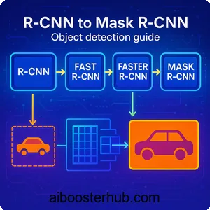
R-CNN to Mask R-CNN: Object detection guide

The evolution of object detection algorithms represents a fascinating journey of innovation in deep learning. Among the most influential breakthroughs in this field are the R-CNN family of algorithms: R-CNN, Fast R-CNN, Faster R-CNN, and Mask R-CNN. These two-stage detection methods revolutionized how we approach object detection by combining region proposal mechanisms with convolutional neural networks (CNN). Each iteration addressed specific bottlenecks of its predecessor, progressively improving both accuracy and speed. In this comprehensive guide, we’ll explore how these algorithms work, their architectural innovations, and how to implement them for practical applications.

1. Understanding object detection fundamentals

Before diving into specific algorithms, it’s essential to understand what makes object detection challenging and different from other computer vision tasks. Object detection requires a model to accomplish two distinct tasks simultaneously: classification (what is the object?) and localization (where is the object?).

The core challenges

The primary challenge in object detection stems from the vast number of possible locations and scales where objects might appear. An object could be anywhere in an image, at any size, and in any orientation. A naive approach might involve sliding a fixed-size window across the entire image at multiple scales, but this becomes computationally prohibitive for high-resolution images.

Additionally, real-world images often contain multiple objects of different categories, overlapping instances, and varying lighting conditions. The algorithm must not only detect each object but also distinguish between closely positioned instances of the same class, a problem known as instance segmentation.

Evaluation metrics

Object detection models are typically evaluated using Intersection over Union (IoU) and mean Average Precision (mAP). IoU measures how much the predicted bounding box overlaps with the ground truth:

$$\text{IoU} = \frac{\text{Area of Overlap}}{\text{Area of Union}}$$​

A detection is considered correct if its IoU exceeds a threshold (commonly 0.5) and the predicted class matches the ground truth. The mAP metric averages the precision across different recall levels and object categories, providing a single number that summarizes model performance.

Two-stage vs one-stage detectors

Object detection algorithms generally fall into two categories: two-stage and one-stage detectors. Two-stage detectors, like the R-CNN family, first generate region proposals (candidate locations where objects might be) and then classify these regions. This approach tends to be more accurate but slower. One-stage detectors, like YOLO and SSD, predict bounding boxes and class probabilities directly in a single pass, trading some accuracy for speed.

The R-CNN family represents the evolution of two-stage detection, where each version introduced innovations that addressed the limitations of earlier approaches while maintaining high accuracy.

2. R-CNN: The pioneering approach

R-CNN (Regions with CNN features) marked a paradigm shift in object detection by effectively applying deep learning to this task. Prior to R-CNN, most object detection systems relied on hand-crafted features and complex pipelines. R-CNN demonstrated that CNN features could dramatically improve detection accuracy.

Architecture overview

R-CNN operates through a multi-stage pipeline. First, it uses selective search, a traditional computer vision algorithm, to generate approximately 2,000 region proposals per image. These proposals are potential bounding boxes where objects might be located. Selective search works by initially segmenting the image and then hierarchically grouping similar regions based on color, texture, size, and shape.

Each region proposal is then warped to a fixed size (typically 227×227 pixels) regardless of its original aspect ratio. This warping is necessary because CNNs require fixed-size inputs. The warped regions are fed through a pre-trained CNN (originally AlexNet) to extract a 4096-dimensional feature vector for each region.

These feature vectors are then classified using class-specific linear Support Vector Machines (SVMs). Finally, a bounding box regressor refines the coordinates of each detection to better fit the actual object boundaries.

Strengths and limitations

R-CNN achieved breakthrough accuracy on benchmark datasets, significantly outperforming previous methods. The use of deep CNN features proved far more effective than hand-crafted features, establishing a new paradigm for object detection.

However, R-CNN has significant drawbacks. Training is a multi-stage process: first training the CNN, then the SVMs, and finally the bounding box regressors. This complexity makes the system difficult to optimize end-to-end. More critically, inference is extremely slow, taking approximately 47 seconds per image on a GPU, because each region proposal must be processed independently through the CNN. The feature extraction stage also requires significant disk space to cache features for all proposals.

3. Fast R-CNN: Streamlining the pipeline

Fast R-CNN addressed the computational inefficiencies of R-CNN while maintaining its accuracy. The key insight was that processing each region proposal independently through a CNN was wasteful, as proposals from the same image share much of their computation.

Key innovations

Fast R-CNN introduces several architectural improvements. Instead of running the CNN on each region proposal, it processes the entire image once to create a feature map. Region proposals are then projected onto this feature map, and a technique called RoI (Region of Interest) pooling extracts fixed-size feature vectors from each region.

RoI pooling works by dividing each region of interest into a grid (typically 7×7) and performing max pooling within each grid cell. This produces a fixed-size output regardless of the input region’s size, eliminating the need for warping and preserving spatial information better than R-CNN’s approach.

Another major innovation is the multi-task loss function that trains classification and bounding box regression simultaneously:

$$L = L_{\text{cls}}(p, u) + \lambda [u \geq 1] \, L_{\text{loc}}(t^u, v)$$

Where \(L_{\text{cls}}\) is the classification loss, \(L_{\text{loc}}\) is the localization loss, \(p\) is the predicted class probability, \(u\) is the true class, \(t^u\) is the predicted bounding box, and \(v\) is the ground truth box. The indicator function \([u \geq 1]\) ensures that bounding box regression is only applied to non-background classes.

Performance improvements

Fast R-CNN achieves dramatic speedups compared to R-CNN. Training time is reduced by approximately 9× because the entire network can be trained end-to-end with a single-stage training process. Inference speed improves by about 213×, processing images in approximately 0.3 seconds instead of 47 seconds.

The accuracy also improves slightly due to the end-to-end training and better feature sharing. However, Fast R-CNN still relies on selective search for region proposals, which runs on the CPU and becomes the bottleneck. Generating proposals takes about 2 seconds per image, dominating the overall detection time.

4. Faster R-CNN: Learning region proposals

Faster R-CNN represents the culmination of the R-CNN evolution by introducing the Region Proposal Network (RPN), which learns to generate proposals directly from the CNN features. This innovation makes the entire detection pipeline fully differentiable and trainable end-to-end.

The Region Proposal Network

The RPN is a small fully convolutional network that slides over the CNN feature map and predicts region proposals at each location. At each position, the RPN considers k anchor boxes of different scales and aspect ratios (typically 9 anchors: 3 scales × 3 aspect ratios). For each anchor, the RPN outputs two values: an objectness score (probability that the region contains an object) and four bounding box regression coordinates.

The RPN architecture consists of a 3×3 convolutional layer followed by two sibling 1×1 convolutional layers: one for classification (2k scores for object/not-object) and one for regression (4k coordinates for box refinement). This lightweight design allows the RPN to share computation with the detection network efficiently.

Training strategy

Faster R-CNN uses a four-step alternating training process. First, the RPN is trained independently using ImageNet-pretrained weights. Second, a separate Fast R-CNN detection network is trained using proposals from the trained RPN. Third, the detector network is used to initialize RPN training, but the shared convolutional layers are frozen. Finally, the shared convolutional layers remain frozen while fine-tuning the unique layers of Fast R-CNN.

Alternatively, an approximate joint training approach can be used where the RPN and detection network are trained simultaneously in a single stage, which is simpler but gives similar results.

Advantages and impact

Faster R-CNN achieves near real-time performance while maintaining high accuracy. The RPN generates proposals in about 10ms per image on a GPU, making it approximately 200× faster than selective search. The entire detection pipeline runs at about 5-17 frames per second depending on the backbone network.

More importantly, Faster R-CNN demonstrated that region proposals could be learned as part of the detection network, eliminating the need for external proposal algorithms. This insight influenced many subsequent detection architectures and established the standard for two-stage detection methods that remains relevant today.

5. Mask R-CNN: Adding instance segmentation

Mask R-CNN extends Faster R-CNN to perform instance segmentation, where the goal is to detect objects and delineate their exact pixel-wise boundaries. This additional capability makes it invaluable for applications requiring precise object localization, such as medical imaging, robotics, and augmented reality.

Architecture extensions

Mask R-CNN adds a third branch to the Faster R-CNN architecture. Alongside the existing classification and bounding box regression branches, it introduces a mask prediction branch that outputs a binary mask for each RoI. The mask branch is a small fully convolutional network that predicts an m×m mask for each RoI.

A crucial innovation in Mask R-CNN is RoIAlign, which replaces the RoI pooling used in Faster R-CNN. RoI pooling performs quantization when mapping RoIs to the feature map, which causes misalignment between the RoI and the extracted features. This misalignment is acceptable for bounding box detection but problematic for pixel-level mask prediction.

RoIAlign eliminates quantization by using bilinear interpolation to compute feature values at exactly four regularly sampled locations in each RoI bin, then aggregating them with max or average pooling. This preserves precise spatial correspondence, leading to significant improvements in mask accuracy.

Multi-task learning

Mask R-CNN is trained with a multi-task loss combining classification, bounding box regression, and mask prediction:

$$L = L_{\text{cls}} + L_{\text{box}} + L_{\text{mask}}$$​

The mask loss is defined as the average binary cross-entropy loss over all pixels:

$$L_{\text{mask}} = -\frac{1}{m^2}
\sum_{1 \leq i, j \leq m}
\left[
y_{ij} \log \hat{y}_{ij}^k + (1 – y_{ij}) \log(1 – \hat{y}_{ij}^k)
\right]$$

Where \(y_{ij}\) is the ground truth mask pixel, \(\hat{y}_{ij}^k\) is the predicted probability at pixel \((i,j)\) for class \(k\), and the loss is computed only for the ground truth class \(k\). This decouples mask and class prediction, allowing the network to generate masks for all classes without competition.

Applications and impact

Mask R-CNN has become the de facto standard for instance segmentation tasks. Its ability to precisely delineate object boundaries enables applications that require detailed understanding of object shapes and positions. Medical imaging applications leverage this precision to segment organs and tumors with remarkable accuracy. Autonomous driving systems benefit from its capability to distinguish between individual vehicles and pedestrians even when they overlap. Retail and warehouse automation deploy the algorithm to enable robots to identify and manipulate individual items efficiently.

The architecture’s flexibility also allows it to be adapted for related tasks. By modifying the mask branch, researchers have extended Mask R-CNN to predict keypoints for human pose estimation, estimate 3D object poses, and even perform panoptic segmentation that unifies instance and semantic segmentation.

6. Practical considerations and best practices

When implementing these object detection algorithms in real-world applications, several practical considerations can significantly impact performance and usability.

Choosing the right algorithm

The choice between R-CNN variants depends on your specific requirements. If accuracy is paramount and computational resources are available, Mask R-CNN with a strong backbone like ResNet-101 or ResNeXt provides state-of-the-art results. For applications requiring real-time performance without instance segmentation, Faster R-CNN with a lighter backbone like MobileNet offers a good balance.

Consider the inference environment carefully. On powerful GPUs, Mask R-CNN can process images in real-time, but on embedded devices or CPUs, even Faster R-CNN might be too slow. In such cases, knowledge distillation or model quantization techniques can help reduce computational requirements while maintaining acceptable accuracy.

Data preparation and augmentation

The quality and quantity of training data significantly impact detection performance. These models typically require thousands of annotated images per category. Data augmentation techniques like random scaling, flipping, color jittering, and random cropping help improve generalization and prevent overfitting.

For bounding box annotations, ensure consistency in how objects are labeled, particularly for partially visible or occluded objects. For instance segmentation, high-quality pixel-level annotations are crucial. Tools like LabelMe, CVAT, or Supervisely can streamline the annotation process.

Transfer learning and fine-tuning

Pre-training on large datasets like COCO or ImageNet provides strong initialization for the backbone network. When fine-tuning for specific domains, use lower learning rates for pre-trained layers and higher rates for newly initialized layers. The detection head and RPN typically require more aggressive learning rates than the backbone.

Handling class imbalance

Object detection datasets often have severe class imbalance, with background regions vastly outnumbering foreground objects. The R-CNN family addresses this through careful sampling of positive and negative examples during training. Typically, each mini-batch contains a 1:3 ratio of positive to negative samples.

Focal loss, introduced for one-stage detectors, can also be applied to R-CNN variants to down-weight easy examples and focus learning on hard cases:

$$ \text{FL}(p_t) = -\alpha_t (1-p_t)^\gamma \log(p_t) $$

Where \(p_t\) is the predicted probability for the true class, \(\alpha_t\) balances positive/negative examples, and \(\gamma\) reduces loss for well-classified examples.

Post-processing and NMS

Non-Maximum Suppression (NMS) removes duplicate detections by suppressing boxes with high IoU overlap with higher-scoring boxes. The NMS threshold requires tuning: lower values (0.3-0.5) produce cleaner results but may suppress valid detections of overlapping objects, while higher values (0.7-0.9) retain more detections but may include duplicates.

7. Conclusion

The evolution from R-CNN to Mask R-CNN represents a remarkable journey of innovation in computer vision, demonstrating how systematic improvements to architecture and training procedures can yield dramatic gains in both accuracy and efficiency. Each iteration addressed specific limitations of its predecessor while maintaining the core insight that deep CNNs can learn powerful representations for object detection.

These algorithms have established the foundation for modern two-stage detection methods and continue to influence current research. Whether you’re building an autonomous vehicle perception system, developing medical image analysis tools, or creating intelligent video surveillance, understanding the R-CNN family provides essential insights into how state-of-the-art object detection works. By mastering these foundational techniques and applying the practical considerations discussed, you’ll be well-equipped to implement robust object detection systems for your specific applications.

8. Knowledge Check

Quiz 1: Object detection vs classification

Question: Explain the key difference between image classification and object detection, and why object detection is more computationally challenging.

Answer: Image classification only identifies what objects are present in an image, while object detection must determine both what objects exist and where they are located. Object detection is more challenging because it requires examining numerous possible locations and scales where objects might appear, making it computationally intensive compared to single-label classification.

Quiz 2: R-CNN architecture

Question: Describe the main components of the original R-CNN pipeline and identify its primary computational bottleneck.

Answer: R-CNN uses selective search to generate approximately 2,000 region proposals, warps each region to a fixed size, extracts CNN features from each region individually, and classifies them using SVMs with bounding box regression. The primary bottleneck is that each region proposal must be processed independently through the CNN, making inference extremely slow at about 47 seconds per image.

Quiz 3: Evaluation metrics

Question: What is Intersection over Union (IoU) and how is it used to evaluate object detection performance?

Answer: IoU measures the overlap between a predicted bounding box and the ground truth box, calculated as the area of overlap divided by the area of union. A detection is considered correct if its IoU exceeds a threshold (typically 0.5) and the predicted class matches the ground truth. This metric is fundamental to computing mean Average Precision (mAP).

Quiz 4: Fast R-CNN innovation

Question: What key architectural change did Fast R-CNN introduce to improve upon R-CNN’s speed, and what technique enables fixed-size feature extraction?

Answer: Fast R-CNN processes the entire image once through the CNN to create a feature map, rather than processing each region proposal separately. It uses RoI (Region of Interest) pooling to extract fixed-size feature vectors from arbitrary-sized regions on the feature map by dividing each region into a grid and performing max pooling within each cell.

Quiz 5: Multi-task loss

Question: Explain the multi-task loss function used in Fast R-CNN and why training both tasks together is beneficial.

Answer: Fast R-CNN uses a combined loss function that trains classification and bounding box regression simultaneously: L = L_cls + λL_loc. This end-to-end training approach is more efficient than R-CNN’s multi-stage training and allows the network to learn shared representations that benefit both tasks, improving overall accuracy while simplifying the training pipeline.

Quiz 6: Region Proposal Network

Question: What problem does the Region Proposal Network (RPN) in Faster R-CNN solve, and how does it generate proposals?

Answer: The RPN eliminates the need for slow external proposal algorithms like selective search by learning to generate region proposals directly from CNN features. It slides over the feature map and predicts objectness scores and bounding box coordinates for multiple anchor boxes at each location, making proposal generation about 200× faster than selective search.

Quiz 7: Anchor boxes

Question: Describe what anchor boxes are in Faster R-CNN and why multiple anchors are used at each location.

Answer: Anchor boxes are pre-defined bounding boxes of various scales and aspect ratios centered at each position in the feature map. Faster R-CNN typically uses 9 anchors per location (3 scales × 3 aspect ratios) to handle objects of different sizes and shapes, allowing the network to detect objects at multiple scales without requiring an image pyramid.

Quiz 8: RoIAlign innovation

Question: Why did Mask R-CNN replace RoI pooling with RoIAlign, and how does RoIAlign work differently?

Answer: RoI pooling performs quantization when mapping regions to the feature map, causing misalignment that’s problematic for pixel-precise mask prediction. RoIAlign eliminates quantization by using bilinear interpolation to compute feature values at exact floating-point locations, preserving precise spatial correspondence essential for accurate instance segmentation.

Quiz 9: Instance segmentation

Question: What additional capability does Mask R-CNN provide beyond Faster R-CNN, and how is the mask branch trained?

Answer: Mask R-CNN adds instance segmentation, which provides pixel-wise object boundaries rather than just bounding boxes. It adds a mask prediction branch that outputs binary masks for each RoI. The mask loss uses binary cross-entropy computed only for the ground truth class, decoupling mask and class prediction to allow independent mask generation for all classes.

Quiz 10: Two-stage vs one-stage detectors

Question: Compare two-stage detectors like the R-CNN family with one-stage detectors, discussing their trade-offs in accuracy and speed.

Answer: Two-stage detectors first generate region proposals then classify them, achieving higher accuracy but slower inference. One-stage detectors like YOLO predict bounding boxes and classes directly in a single pass, offering faster processing but typically lower accuracy. The R-CNN family represents the evolution of two-stage detection, progressively improving both speed and accuracy through architectural innovations.