Recurrent Neural Networks (RNN): Complete Guide
Understanding sequential data is fundamental to artificial intelligence. From language translation to stock price prediction, many real-world problems involve data that flows through time. This is where recurrent neural networks come into play—a specialized class of neural networks designed specifically for temporal processing and sequence modeling.

Content
Toggle1. What is a recurrent neural network?
A recurrent neural network (RNN) is a type of artificial neural network (ANN) designed to recognize patterns in sequences of data. Unlike traditional feedforward neural networks, RNNs have connections that loop back on themselves, allowing them to maintain an internal memory of previous inputs. This recurrent structure makes them exceptionally powerful for tasks involving sequential data.
The RNN full form is “Recurrent Neural Network,” and the term “recurrent” carries significant meaning. The recurrent definition refers to something that occurs repeatedly or returns periodically. In the context of neural networks, recurrent meaning describes the network’s ability to use outputs from previous steps as inputs for current computations—creating a feedback loop that enables the network to “remember” past information.
What makes RNNs unique?
Traditional neural networks process each input independently, with no memory of previous inputs. Imagine reading a book where you forget every sentence immediately after reading it—you’d struggle to understand the story. RNNs solve this problem by maintaining hidden states that act as memory, allowing them to consider context from earlier in the sequence.
Consider this practical example: when you type on your smartphone, the autocomplete feature predicts the next word based on what you’ve already typed. An RNN model powers this functionality by processing your text sequentially, maintaining context about previous words to make intelligent predictions about what comes next.
2. Understanding RNN architecture
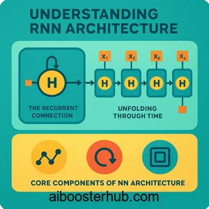
The RNN architecture distinguishes itself through its unique structure that enables sequential modeling. At its core, an RNN processes sequences one element at a time while maintaining a hidden state that captures information from previous time steps.
Core components of RNN architecture
An RNN consists of three primary components:
- Input layer: Receives sequential data at each time step
- Hidden layer: Maintains the network’s memory through recurrent connections
- Output layer: Produces predictions based on current input and hidden state
The mathematical foundation of an RNN can be expressed through these equations:
$$h_t = \tanh(W_{hh} h_{t-1} + W_{xh} x_t + b_h)$$
$$y_t = W_{hy} h_t + b_y$$
Where:
- \(h_t\) represents the hidden state at time step \(t\)
- \(x_t\) is the input at time step \(t\)
- \(y_t\) is the output at time step \(t\)
- \(W_{hh}\), \(W_{xh}\), and \(W_{hy}\) are weight matrices
- \(b_h\) and \(b_y\) are bias vectors
- \(\tanh\) is the activation function
The recurrent connection
What makes RNNs truly “recurrent” is the connection from the hidden layer back to itself. This feedback loop allows information to persist across time steps. When processing a sequence, the hidden state at time \(t\) depends both on the current input and the hidden state from time \(t-1\), creating a chain of dependencies through time.
Here’s a simple Python implementation demonstrating the basic RNN computation:
import numpy as np

def rnn_step(x, h_prev, Wxh, Whh, Why, bh, by):
    """
    Single step of RNN forward pass
    x: input at current time step (vector)
    h_prev: hidden state from previous time step
    """
    # Compute new hidden state
    h = np.tanh(np.dot(Wxh, x) + np.dot(Whh, h_prev) + bh)

    # Compute output
    y = np.dot(Why, h) + by

    return h, y

# Example usage
input_size = 10
hidden_size = 20
output_size = 5

# Initialize weights randomly
Wxh = np.random.randn(hidden_size, input_size) * 0.01
Whh = np.random.randn(hidden_size, hidden_size) * 0.01
Why = np.random.randn(output_size, hidden_size) * 0.01
bh = np.zeros((hidden_size, 1))
by = np.zeros((output_size, 1))

# Process a sequence
sequence_length = 7
h = np.zeros((hidden_size, 1))  # Initial hidden state

for t in range(sequence_length):
    x = np.random.randn(input_size, 1)  # Input at time t
    h, y = rnn_step(x, h, Wxh, Whh, Why, bh, by)
    print(f"Time step {t}: output shape = {y.shape}")
Unfolding through time
To better understand how RNNs process sequences, we can visualize them as “unfolded” through time. This unfolding shows the same network structure repeated at each time step, with connections between consecutive time steps representing the recurrent connections.
3. Types of RNN models and variants
While the basic RNN provides a foundation for sequential modeling, several advanced variants have been developed to address specific challenges and improve performance in RNN deep learning applications.
Long Short-Term Memory (LSTM)
LSTM networks are the most popular RNN variant, designed to solve the vanishing gradient problem that plagues standard RNNs. They introduce a more complex cell structure with gates that control information flow:
- Forget gate: Decides what information to discard from the cell state
- Input gate: Determines what new information to store
- Output gate: Controls what information to output
The LSTM equations are:
$$f_t = \sigma(W_f \cdot [h_{t-1}, x_t] + b_f)$$
$$i_t = \sigma(W_i \cdot [h_{t-1}, x_t] + b_i)$$
$$\tilde{C}_t = \tanh(W_C \cdot [h_{t-1}, x_t] + b_C)$$
$$C_t = f_t \ast C_{t-1} + i_t \ast \tilde{C}_t$$
$$o_t = \sigma(W_o \cdot [h_{t-1}, x_t] + b_o)$$
$$h_t = o_t \ast \tanh(C_t)$$
Here’s a practical LSTM implementation using Python:
import numpy as np

class SimpleLSTM:
    def __init__(self, input_size, hidden_size):
        self.hidden_size = hidden_size

        # Initialize weights for all gates
        self.Wf = np.random.randn(hidden_size, input_size + hidden_size) * 0.01
        self.Wi = np.random.randn(hidden_size, input_size + hidden_size) * 0.01
        self.Wc = np.random.randn(hidden_size, input_size + hidden_size) * 0.01
        self.Wo = np.random.randn(hidden_size, input_size + hidden_size) * 0.01

        # Initialize biases
        self.bf = np.zeros((hidden_size, 1))
        self.bi = np.zeros((hidden_size, 1))
        self.bc = np.zeros((hidden_size, 1))
        self.bo = np.zeros((hidden_size, 1))

    def sigmoid(self, x):
        return 1 / (1 + np.exp(-x))

    def forward_step(self, x, h_prev, c_prev):
        # Concatenate input and previous hidden state
        combined = np.vstack((h_prev, x))

        # Forget gate
        f = self.sigmoid(np.dot(self.Wf, combined) + self.bf)

        # Input gate
        i = self.sigmoid(np.dot(self.Wi, combined) + self.bi)

        # Candidate cell state
        c_tilde = np.tanh(np.dot(self.Wc, combined) + self.bc)

        # New cell state
        c = f * c_prev + i * c_tilde

        # Output gate
        o = self.sigmoid(np.dot(self.Wo, combined) + self.bo)

        # New hidden state
        h = o * np.tanh(c)

        return h, c

# Example usage
lstm = SimpleLSTM(input_size=10, hidden_size=20)
h = np.zeros((20, 1))
c = np.zeros((20, 1))

x = np.random.randn(10, 1)
h_new, c_new = lstm.forward_step(x, h, c)
print(f"New hidden state shape: {h_new.shape}")
print(f"New cell state shape: {c_new.shape}")
Gated Recurrent Unit (GRU)
GRU is a simplified version of LSTM with fewer parameters, making it computationally more efficient while maintaining similar performance. It combines the forget and input gates into a single “update gate” and merges the cell state and hidden state.
Bidirectional RNNs
Bidirectional RNNs process sequences in both forward and backward directions, allowing the network to capture context from both past and future. This is particularly useful for tasks like speech recognition or text classification where the entire sequence is available during processing.
Deep RNNs
Deep RNNs stack multiple recurrent layers on top of each other, allowing the network to learn hierarchical representations of sequential data. Each layer processes the output sequence from the layer below it.
4. How RNN deep learning works
Understanding how RNNs learn from sequential data requires examining both the forward pass (how predictions are made) and the backward pass (how the network learns from errors).
Forward propagation through time
During forward propagation, the RNN processes the input sequence one element at a time. At each time step \(t\):
- The network receives input \(x_t\)
- It combines this input with the hidden state from the previous step \(h_{t-1}\)
- It computes a new hidden state \(h_t\)
- It produces an output \(y_t\)
This process continues until the entire sequence is processed. The key insight is that the same set of weights is used at every time step—the network learns a single set of parameters that works across the entire sequence.
Backpropagation through time (BPTT)
Training RNNs uses a specialized version of backpropagation called Backpropagation Through Time (BPTT). The network is “unfolded” through time, and gradients are computed by flowing backward through all time steps.
The gradient of the loss with respect to a weight is the sum of gradients at each time step:
$$\frac{\partial L}{\partial W} = \sum_{t=1}^{T} \frac{\partial L_t}{\partial W}$$
Here’s a simplified implementation of BPTT:
import numpy as np

def bptt(inputs, targets, h_init, Wxh, Whh, Why, bh, by):
    """
    Simplified backpropagation through time
    inputs: list of input vectors
    targets: list of target outputs
    """
    # Forward pass
    xs, hs, ys, ps = {}, {}, {}, {}
    hs[-1] = np.copy(h_init)
    loss = 0

    # Forward pass through sequence
    for t in range(len(inputs)):
        xs[t] = inputs[t]
        hs[t] = np.tanh(np.dot(Wxh, xs[t]) + np.dot(Whh, hs[t-1]) + bh)
        ys[t] = np.dot(Why, hs[t]) + by
        ps[t] = np.exp(ys[t]) / np.sum(np.exp(ys[t]))  # Softmax
        loss += -np.log(ps[t][targets[t], 0])

    # Backward pass: compute gradients
    dWxh = np.zeros_like(Wxh)
    dWhh = np.zeros_like(Whh)
    dWhy = np.zeros_like(Why)
    dbh = np.zeros_like(bh)
    dby = np.zeros_like(by)
    dh_next = np.zeros_like(hs[0])

    # Backward through time
    for t in reversed(range(len(inputs))):
        dy = np.copy(ps[t])
        dy[targets[t]] -= 1  # Gradient of loss w.r.t. output

        dWhy += np.dot(dy, hs[t].T)
        dby += dy

        dh = np.dot(Why.T, dy) + dh_next
        dh_raw = (1 - hs[t] * hs[t]) * dh  # Backprop through tanh

        dbh += dh_raw
        dWxh += np.dot(dh_raw, xs[t].T)
        dWhh += np.dot(dh_raw, hs[t-1].T)
        dh_next = np.dot(Whh.T, dh_raw)

    # Clip gradients to prevent exploding gradients
    for dparam in [dWxh, dWhh, dWhy, dbh, dby]:
        np.clip(dparam, -5, 5, out=dparam)

    return loss, dWxh, dWhh, dWhy, dbh, dby
Challenges in training RNNs
Training RNNs presents unique challenges:
Vanishing gradients: When backpropagating through many time steps, gradients can become exponentially small, making it difficult for the network to learn long-term dependencies. This is why LSTM and GRU architectures were developed.
Exploding gradients: Conversely, gradients can also become exponentially large, causing the network weights to update too drastically. Gradient clipping (as shown in the code above) is a common solution.
Computational cost: BPTT requires storing activations for all time steps, making memory consumption proportional to sequence length.
5. Practical applications of recurrent neural networks
Recurrent neural networks excel in numerous domains where sequential modeling and temporal processing are essential. Their ability to maintain memory across time steps makes them invaluable for real-world applications.
Natural language processing
RNNs have revolutionized how machines understand and generate human language:
Language modeling: RNNs predict the next word in a sequence, enabling applications like autocomplete and text generation. For example, when you start typing an email, the suggestions you see are often powered by RNN-based language models.
Machine translation: Sequence-to-sequence models using RNNs can translate text from one language to another. The encoder RNN processes the source language sentence into a fixed representation, and the decoder RNN generates the translation.
Sentiment analysis: RNNs analyze the sentiment of text by processing words sequentially and maintaining context throughout the document.
Here’s a simple character-level text generation example:
import numpy as np

class CharRNN:
    def __init__(self, vocab_size, hidden_size):
        self.vocab_size = vocab_size
        self.hidden_size = hidden_size

        # Initialize parameters
        self.Wxh = np.random.randn(hidden_size, vocab_size) * 0.01
        self.Whh = np.random.randn(hidden_size, hidden_size) * 0.01
        self.Why = np.random.randn(vocab_size, hidden_size) * 0.01
        self.bh = np.zeros((hidden_size, 1))
        self.by = np.zeros((vocab_size, 1))

    def sample(self, h, seed_ix, n):
        """
        Generate a sequence of characters
        h: initial hidden state
        seed_ix: seed letter for first time step
        n: number of characters to generate
        """
        x = np.zeros((self.vocab_size, 1))
        x[seed_ix] = 1
        generated_chars = []

        for t in range(n):
            h = np.tanh(np.dot(self.Wxh, x) + np.dot(self.Whh, h) + self.bh)
            y = np.dot(self.Why, h) + self.by
            p = np.exp(y) / np.sum(np.exp(y))

            # Sample from probability distribution
            ix = np.random.choice(range(self.vocab_size), p=p.ravel())

            # Update input for next time step
            x = np.zeros((self.vocab_size, 1))
            x[ix] = 1
            generated_chars.append(ix)

        return generated_chars

# Example usage
vocab_size = 27  # 26 letters + space
hidden_size = 100
model = CharRNN(vocab_size, hidden_size)

# Generate 50 characters
h = np.zeros((hidden_size, 1))
sequence = model.sample(h, seed_ix=0, n=50)
print(f"Generated sequence length: {len(sequence)}")
Time series prediction
RNNs are naturally suited for analyzing temporal data:
Stock market forecasting: By processing historical price data sequentially, RNNs can identify patterns and predict future price movements.
Weather prediction: RNNs analyze meteorological time series data to forecast weather conditions.
Energy consumption forecasting: Utility companies use RNNs to predict electricity demand based on historical usage patterns.
Speech and audio processing
Speech recognition: RNNs convert spoken words into text by processing audio signals as sequences of acoustic features. Modern voice assistants rely heavily on RNN-based models.
Music generation: By learning patterns in musical sequences, RNNs can compose original music in various styles.
Audio classification: RNNs can identify specific sounds or events in audio streams, useful for applications like sound-based surveillance or environmental monitoring.
Video analysis
Action recognition: RNNs process video frames sequentially to recognize human actions and activities.
Video captioning: By combining convolutional neural networks (for visual features) with RNNs (for sequence generation), systems can automatically generate descriptions of video content.
6. Implementing RNNs: Best practices and considerations
Successfully deploying RNN models in production requires careful attention to architecture choices, hyperparameters, and training strategies.
Choosing the right architecture
The choice between vanilla RNN, LSTM, and GRU depends on your specific use case:
Use vanilla RNNs when dealing with short sequences and simple patterns. They’re computationally efficient but struggle with long-term dependencies.
Choose LSTM when you need to capture long-term dependencies and have sufficient computational resources. LSTMs are more expressive but require more memory and training time.
Select GRU when you want a balance between performance and efficiency. GRUs are faster to train than LSTMs while still handling long-term dependencies effectively.
Hyperparameter tuning
Critical hyperparameters for RNNs include:
Hidden layer size: Determines the network’s capacity to learn complex patterns. Start with 128-512 units and adjust based on performance.
Number of layers: Deeper networks can learn more abstract representations. Two to three layers often work well for most applications.
Learning rate: Typically ranges from 0.001 to 0.01 for Adam optimizer. Use learning rate scheduling to improve convergence.
Sequence length: Longer sequences provide more context but increase computational cost. Experiment with different truncation lengths.
Here’s a complete LSTM implementation for sequence classification:
import numpy as np

class LSTMClassifier:
    def __init__(self, input_size, hidden_size, output_size, learning_rate=0.001):
        self.hidden_size = hidden_size
        self.lr = learning_rate

        # Initialize weights
        self.Wf = np.random.randn(hidden_size, input_size + hidden_size) * 0.01
        self.Wi = np.random.randn(hidden_size, input_size + hidden_size) * 0.01
        self.Wc = np.random.randn(hidden_size, input_size + hidden_size) * 0.01
        self.Wo = np.random.randn(hidden_size, input_size + hidden_size) * 0.01
        self.Wy = np.random.randn(output_size, hidden_size) * 0.01

        # Initialize biases
        self.bf = np.zeros((hidden_size, 1))
        self.bi = np.zeros((hidden_size, 1))
        self.bc = np.zeros((hidden_size, 1))
        self.bo = np.zeros((hidden_size, 1))
        self.by = np.zeros((output_size, 1))

    def sigmoid(self, x):
        return 1 / (1 + np.exp(-np.clip(x, -500, 500)))

    def softmax(self, x):
        exp_x = np.exp(x - np.max(x))
        return exp_x / np.sum(exp_x)

    def forward(self, inputs):
        """
        Forward pass through the LSTM
        inputs: sequence of input vectors
        """
        T = len(inputs)
        h = np.zeros((self.hidden_size, 1))
        c = np.zeros((self.hidden_size, 1))

        # Store states for backprop
        self.cache = {
            'inputs': inputs,
            'h_states': [h],
            'c_states': [c],
            'gates': []
        }

        # Process sequence
        for t in range(T):
            x = inputs[t].reshape(-1, 1)
            combined = np.vstack((h, x))

            # Gates
            f = self.sigmoid(np.dot(self.Wf, combined) + self.bf)
            i = self.sigmoid(np.dot(self.Wi, combined) + self.bi)
            c_tilde = np.tanh(np.dot(self.Wc, combined) + self.bc)
            o = self.sigmoid(np.dot(self.Wo, combined) + self.bo)

            # Update states
            c = f * c + i * c_tilde
            h = o * np.tanh(c)

            self.cache['h_states'].append(h)
            self.cache['c_states'].append(c)
            self.cache['gates'].append((f, i, c_tilde, o))

        # Final classification
        output = np.dot(self.Wy, h) + self.by
        probs = self.softmax(output)

        return probs

    def train_step(self, inputs, target):
        """
        Single training step
        inputs: sequence of input vectors
        target: target class (integer)
        """
        # Forward pass
        probs = self.forward(inputs)

        # Compute loss
        loss = -np.log(probs[target, 0] + 1e-8)

        # Backward pass would go here
        # (simplified for brevity)

        return loss, probs

# Example usage
input_size = 10
hidden_size = 50
output_size = 3  # 3 classes
sequence_length = 20

model = LSTMClassifier(input_size, hidden_size, output_size)

# Create random sequence
sequence = [np.random.randn(input_size) for _ in range(sequence_length)]
target_class = 1

loss, probs = model.train_step(sequence, target_class)
print(f"Loss: {loss:.4f}")
print(f"Predicted probabilities: {probs.ravel()}")
Regularization techniques
Preventing overfitting is crucial for RNN performance:
Dropout: Apply dropout to input connections and recurrent connections separately. Typical dropout rates range from 0.2 to 0.5.
Weight regularization: Add L2 regularization to prevent weights from growing too large.
Early stopping: Monitor validation loss and stop training when it starts increasing.
Gradient clipping: Clip gradients by norm to prevent exploding gradients, typically to a maximum norm of 5-10.
Practical implementation tips
When building RNN applications, consider these guidelines:
Start simple: Begin with a small model and gradually increase complexity. This helps identify issues early and reduces debugging time.
Normalize inputs: Scale input features to have zero mean and unit variance. This improves training stability.
Use pretrained embeddings: For NLP tasks, initialize word embeddings with pretrained vectors like Word2Vec or GloVe.
Monitor gradients: Track gradient norms during training. If they consistently spike or vanish, adjust your architecture or hyperparameters.
Batch processing: Process multiple sequences simultaneously to improve computational efficiency.
7. Conclusion
Recurrent neural networks represent a fundamental advancement in how machines process sequential data and perform temporal processing. Through their unique architecture that maintains memory across time steps, RNNs have enabled breakthroughs in natural language processing, time series analysis, speech recognition, and countless other domains requiring sequence modeling.
Understanding what is RNN, how the RNN architecture functions, and when to apply different RNN models provides a solid foundation for tackling sequential data problems. While training challenges like vanishing gradients initially limited their effectiveness, modern variants like LSTM and GRU have largely overcome these obstacles. As you continue exploring neural networks explained in depth, remember that mastering RNNs and their applications in RNN deep learning opens doors to solving complex real-world problems where temporal relationships and sequential patterns are paramount.


