RNN vs CNN: Key differences in deep learning
Artificial neural networks have revolutionized the field of artificial intelligence, enabling machines to learn complex patterns from data. Among the various neural network architectures, Convolutional Neural Networks (CNN) and Recurrent Neural Networks (RNN) stand out as two of the most influential designs. While both are powerful tools in deep learning, they serve fundamentally different purposes and excel at different types of tasks. Understanding the differences between CNN vs RNN is crucial for anyone working with AI and machine learning.

In this comprehensive guide, we’ll explore what makes these architectures unique, their strengths and weaknesses, and how to choose the right one for your specific use case.
1. What is an artificial neural network (ANN)?
Before diving into CNN vs RNN comparisons, let’s establish a foundation by understanding what an artificial neural network (ANN) is. An ANN is a computational model inspired by the biological neural networks in animal brains. The ANN full form refers to “Artificial Neural Network,” which consists of interconnected nodes (neurons) organized in layers.
Basic structure of an ANN model
The typical ANN model contains three types of layers:
- Input Layer: Receives the raw data or features
- Hidden Layers: Process information through weighted connections
- Output Layer: Produces the final prediction or classification
Each connection between neurons has a weight that gets adjusted during training through a process called backpropagation. The network learns by minimizing the difference between predicted outputs and actual targets.
How neural networks learn
The learning process in an ANN involves:
- Forward propagation: Data flows through the network to generate predictions
- Loss calculation: Measuring how far predictions are from actual values
- Backpropagation: Computing gradients to adjust weights
- Weight update: Using optimization algorithms like gradient descent
Here’s a simple example of a basic neural network in Python:
import numpy as np

class SimpleANN:
    def __init__(self, input_size, hidden_size, output_size):
        # Initialize weights randomly
        self.W1 = np.random.randn(input_size, hidden_size)
        self.W2 = np.random.randn(hidden_size, output_size)

    def sigmoid(self, x):
        return 1 / (1 + np.exp(-x))

    def forward(self, X):
        # Forward propagation
        self.z1 = np.dot(X, self.W1)
        self.a1 = self.sigmoid(self.z1)
        self.z2 = np.dot(self.a1, self.W2)
        output = self.sigmoid(self.z2)
        return output

# Example usage
ann = SimpleANN(input_size=3, hidden_size=4, output_size=2)
input_data = np.array([[0.5, 0.3, 0.8]])
prediction = ann.forward(input_data)
print(f"Prediction: {prediction}")
Understanding the ANN forms the basis for comprehending more complex architectures like deep neural networks (DNN), CNN, and RNN.
2. What is RNN? Understanding recurrent neural networks
Now let’s explore what is RNN and why it’s essential in deep learning. RNN stands for Recurrent Neural Network (the RNN full form), a type of neural network designed specifically to work with sequential data.
RNN architecture and how it works
Unlike traditional feedforward neural networks, RNN architecture incorporates loops that allow information to persist. This creates a form of memory, enabling the network to maintain information about previous inputs while processing new ones.
The fundamental equation of an RNN can be expressed as:
$$h_t = \tanh(W_{hh}h_{t-1} + W_{xh}x_t + b_h)$$
$$y_t = W_{hy}h_t + b_y$$
Where:
- \(h_t\) is the hidden state at time step \(t\)
- \(x_t\) is the input at time step \(t\)
- \(y_t\) is the output at time step \(t\)
- \(W_{hh}\), \(W_{xh}\), \(W_{hy}\) are weight matrices
- \(b_h\), \(b_y\) are bias vectors
Key characteristics of RNN deep learning
The RNN’s ability to handle sequential data makes it powerful for:
- Temporal dependencies: Capturing relationships across time steps
- Variable-length inputs: Processing sequences of different lengths
- Shared parameters: Using the same weights across all time steps
- Memory mechanism: Maintaining context from previous inputs
Here’s a practical implementation of a basic RNN:
import numpy as np

class BasicRNN:
    def __init__(self, input_size, hidden_size, output_size):
        self.hidden_size = hidden_size

        # Initialize weights
        self.Wxh = np.random.randn(input_size, hidden_size) * 0.01
        self.Whh = np.random.randn(hidden_size, hidden_size) * 0.01
        self.Why = np.random.randn(hidden_size, output_size) * 0.01

        # Initialize biases
        self.bh = np.zeros((1, hidden_size))
        self.by = np.zeros((1, output_size))

    def forward(self, inputs):
        """
        inputs: list of input vectors (sequence)
        """
        h = np.zeros((1, self.hidden_size))
        outputs = []

        # Process each time step
        for x in inputs:
            # Update hidden state
            h = np.tanh(np.dot(x, self.Wxh) + np.dot(h, self.Whh) + self.bh)
            # Compute output
            y = np.dot(h, self.Why) + self.by
            outputs.append(y)

        return outputs, h

# Example: Processing a sequence
rnn = BasicRNN(input_size=5, hidden_size=10, output_size=3)
sequence = [np.random.randn(1, 5) for _ in range(4)]  # Sequence of 4 time steps
outputs, final_hidden = rnn.forward(sequence)
print(f"Number of outputs: {len(outputs)}")
Applications of RNN
RNNs excel in tasks involving sequential data:
- Natural Language Processing: Text generation, machine translation, sentiment analysis
- Speech Recognition: Converting audio to text
- Time Series Forecasting: Stock prices, weather prediction
- Video Analysis: Action recognition, video captioning
Limitations of basic RNN
While powerful, standard RNNs face challenges:
- Vanishing gradient problem: Difficulty learning long-term dependencies
- Exploding gradients: Unstable training with very long sequences
- Computational inefficiency: Sequential processing limits parallelization
These limitations led to the development of advanced variants like Long Short-Term Memory (LSTM) and Gated Recurrent Units (GRU), which better handle long-term dependencies.
3. What is CNN? Exploring convolutional neural networks
Let’s examine what is CNN and how it differs from RNN. CNN stands for Convolutional Neural Network (the CNN full form), an architecture specifically designed for processing grid-like data, particularly images.
CNN architecture fundamentals
These AI systems use specialized layers that apply convolution operations to extract features from input data. The core components include:
- Convolutional Layers: Apply filters to detect patterns like edges, textures, and shapes
- Pooling Layers: Reduce spatial dimensions while retaining important features
- Fully Connected Layers: Combine features for final classification or prediction
The convolution operation can be mathematically expressed as:
$$S(i,j) = (I * K)(i,j) = \sum_m \sum_n I(m,n)K(i-m, j-n)$$
Where:
- \(S\) is the output feature map
- \(I\) is the input image
- \(K\) is the kernel (filter)
- \(*\) denotes the convolution operation
How CNN processes data
CNNs work through a hierarchical feature extraction process:
- Early layers detect simple features (edges, corners)
- Middle layers combine simple features into complex patterns
- Deep layers recognize high-level concepts (objects, faces)
Here’s a practical CNN implementation:
import numpy as np

class SimpleCNN:
    def __init__(self):
        # Initialize a simple 3x3 edge detection filter
        self.kernel = np.array([[-1, -1, -1],
                                [0,  0,  0],
                                [1,  1,  1]])

    def convolve2d(self, image, kernel):
        """
        Perform 2D convolution
        """
        i_height, i_width = image.shape
        k_height, k_width = kernel.shape

        # Calculate output dimensions
        out_height = i_height - k_height + 1
        out_width = i_width - k_width + 1

        output = np.zeros((out_height, out_width))

        # Perform convolution
        for i in range(out_height):
            for j in range(out_width):
                region = image[i:i+k_height, j:j+k_width]
                output[i, j] = np.sum(region * kernel)

        return output

    def relu(self, x):
        """Activation function"""
        return np.maximum(0, x)

    def max_pool(self, feature_map, pool_size=2):
        """
        Max pooling operation
        """
        h, w = feature_map.shape
        out_h = h // pool_size
        out_w = w // pool_size

        output = np.zeros((out_h, out_w))

        for i in range(out_h):
            for j in range(out_w):
                region = feature_map[i*pool_size:(i+1)*pool_size,
                                    j*pool_size:(j+1)*pool_size]
                output[i, j] = np.max(region)

        return output

    def forward(self, image):
        """
        Forward pass through CNN
        """
        # Convolution
        conv_output = self.convolve2d(image, self.kernel)
        # Activation
        activated = self.relu(conv_output)
        # Pooling
        pooled = self.max_pool(activated)

        return pooled

# Example usage
cnn = SimpleCNN()
# Create a sample 8x8 image
sample_image = np.random.randn(8, 8)
result = cnn.forward(sample_image)
print(f"Input shape: {sample_image.shape}")
print(f"Output shape: {result.shape}")
CNN AI applications
CNNs have transformed computer vision and beyond:
- Image Classification: Recognizing objects in photos
- Object Detection: Locating and identifying multiple objects
- Face Recognition: Identifying individuals from facial features
- Medical Imaging: Detecting diseases in X-rays and MRIs
- Autonomous Vehicles: Processing camera feeds for navigation
Advantages of CNN
- Parameter sharing: Same filter applied across the entire image reduces parameters
- Translation invariance: Detects features regardless of position
- Hierarchical learning: Automatically learns feature hierarchy
- Efficient processing: Convolution operations are computationally efficient
4. CNN vs RNN: Key architectural differences
Now that we understand both architectures, let’s directly compare CNN vs RNN to highlight their fundamental differences.
Data processing approach
CNN:
- Processes spatial data in parallel
- Uses local connectivity and weight sharing
- Excels with grid-structured data (images, videos)
- No inherent temporal dependency handling
RNN:
- Processes sequential data step-by-step
- Maintains hidden state across time steps
- Excels with temporal or sequential data (text, audio)
- Explicitly designed for temporal dependencies
Network topology
The structural difference between CNN RNN architectures is profound:
# CNN structure - processes entire image at once
def cnn_forward(image):
    """
    CNN processes all spatial locations simultaneously
    """
    conv1 = conv_layer(image)          # Parallel processing
    pool1 = max_pool(conv1)            # Downsample
    conv2 = conv_layer(pool1)          # More features
    output = fully_connected(conv2)    # Classification
    return output

# RNN structure - processes sequence step-by-step
def rnn_forward(sequence):
    """
    RNN processes one element at a time, maintaining state
    """
    hidden_state = initialize_hidden()
    outputs = []

    for time_step in sequence:
        hidden_state = rnn_cell(time_step, hidden_state)  # Sequential
        output = compute_output(hidden_state)
        outputs.append(output)

    return outputs
Parameter efficiency
CNN:
- Shared weights across spatial dimensions
- Number of parameters independent of input size
- Typically fewer parameters than RNN for comparable tasks
RNN:
- Shared weights across temporal dimension
- Fixed number of parameters regardless of sequence length
- Can become parameter-heavy with large hidden states
Training characteristics
| Aspect | CNN | RNN |
|---|---|---|
| Parallelization | Highly parallelizable | Limited parallelization |
| Training Speed | Generally faster | Slower due to sequential nature |
| Gradient Flow | More stable | Prone to vanishing/exploding gradients |
| Memory Usage | Moderate | Higher (stores all hidden states) |
Information flow
The way information flows through these networks differs fundamentally:
$$\text{CNN: } y = f(W * x + b)$$
$$\text{RNN: } h_t = f(W_h h_{t-1} + W_x x_t + b)$$
Where CNN applies the same operation across spatial dimensions, while RNN maintains and updates state across time.
5. When to use CNN vs RNN: Practical guidance
Choosing between CNN and RNN depends on your data type and task requirements. Here’s practical guidance for making this decision.
Use CNN when working with:
Spatial data with local patterns
- Image classification and object detection
- Facial recognition systems
- Medical image analysis
- Satellite imagery processing
Example scenario: Building an image classifier for identifying different types of plants.
import numpy as np

class PlantClassifierCNN:
    """
    CNN for plant classification
    Processes spatial features in plant images
    """
    def __init__(self, num_classes=10):
        self.num_classes = num_classes
        # Initialize CNN layers

    def preprocess_image(self, image):
        """
        Prepare image for CNN
        """
        # Resize to fixed dimensions
        # Normalize pixel values
        # Data augmentation if needed
        return processed_image

    def predict(self, image):
        """
        Classify plant species from image
        """
        # CNN processes entire image simultaneously
        features = self.extract_features(image)
        classification = self.classify(features)
        return classification
Data where position matters but not order
- Pattern recognition in fixed-size inputs
- Texture analysis
- Feature extraction from images
Tasks requiring translation invariance
- Detecting objects regardless of location
- Identifying patterns in different positions
Use RNN when working with:
Sequential or temporal data
- Text processing and natural language understanding
- Speech recognition and generation
- Time series forecasting
- Music generation
Example scenario: Sentiment analysis on customer reviews.
class SentimentAnalyzerRNN:
    """
    RNN for analyzing sentiment in text sequences
    """
    def __init__(self, vocab_size, embedding_dim, hidden_dim):
        self.vocab_size = vocab_size
        self.embedding_dim = embedding_dim
        self.hidden_dim = hidden_dim

    def process_review(self, review_text):
        """
        Process review word by word
        """
        words = self.tokenize(review_text)
        hidden_state = self.initialize_hidden()

        # Process each word in sequence
        for word in words:
            word_embedding = self.embed(word)
            hidden_state = self.rnn_step(word_embedding, hidden_state)

        # Final hidden state contains context of entire review
        sentiment = self.classify_sentiment(hidden_state)
        return sentiment  # positive, negative, or neutral
Variable-length inputs
- Sentences of different lengths
- Audio clips of varying duration
- Time series with different time spans
Tasks requiring context from history
- Machine translation
- Video captioning
- Predicting next word in a sentence
Hybrid approaches: Combining CNN and RNN
Sometimes the best solution uses both architectures:
Video analysis: CNN extracts spatial features from frames, RNN processes temporal sequence
class VideoClassifier:
    """
    Hybrid CNN-RNN for video classification
    """
    def __init__(self):
        self.cnn = FeatureExtractorCNN()  # Extract features from frames
        self.rnn = TemporalProcessorRNN()  # Process sequence of features

    def classify_video(self, video_frames):
        """
        Combine CNN and RNN for video understanding
        """
        frame_features = []

        # Use CNN to extract features from each frame
        for frame in video_frames:
            features = self.cnn.extract_features(frame)
            frame_features.append(features)

        # Use RNN to understand temporal relationships
        video_representation = self.rnn.process_sequence(frame_features)
        classification = self.classify(video_representation)

        return classification
Image captioning: CNN encodes image, RNN generates descriptive text
Document classification: CNN extracts local n-gram features, RNN captures long-range dependencies
Decision flowchart
Here’s a simple decision process:
- Is your data grid-like (images, 2D/3D structures)? → Use CNN
- Is your data sequential (text, time series, audio)? → Use RNN
- Do you have both spatial and temporal components? → Consider hybrid CNN-RNN
- Is order important in your data? → RNN; If not → CNN
- Do you need to process variable-length sequences? → RNN
6. Deep neural networks (DNN) and modern variants
While understanding CNN vs RNN is crucial, it’s important to recognize that modern deep learning often uses enhanced versions and combinations of these architectures.
Evolution from ANN to DNN
Deep Neural Networks (DNN) refer to neural networks with multiple hidden layers. Both CNN and RNN can be considered types of DNNs when they have sufficient depth:
- Deep CNN: Multiple convolutional and pooling layers stacked together
- Deep RNN: Multiple recurrent layers processing sequences at different levels of abstraction
The depth allows these networks to learn increasingly abstract representations:
$$\text{Layer 1} \rightarrow \text{Simple features} \rightarrow \text{Layer 2} \rightarrow \text{Complex patterns} \rightarrow \text{Layer N} \rightarrow \text{High-level concepts}$$
Advanced RNN variants
Standard RNNs have evolved into more sophisticated architectures:
LSTM (Long Short-Term Memory)
- Solves vanishing gradient problem
- Better at capturing long-term dependencies
- Uses gates to control information flow
class LSTMCell:
    """
    LSTM cell with forget, input, and output gates
    """
    def forward(self, x_t, h_prev, c_prev):
        """
        LSTM forward pass
        x_t: current input
        h_prev: previous hidden state
        c_prev: previous cell state
        """
        # Forget gate: decides what to forget from cell state
        f_t = self.sigmoid(self.W_f @ [h_prev, x_t] + self.b_f)

        # Input gate: decides what new information to store
        i_t = self.sigmoid(self.W_i @ [h_prev, x_t] + self.b_i)
        c_tilde = self.tanh(self.W_c @ [h_prev, x_t] + self.b_c)

        # Update cell state
        c_t = f_t * c_prev + i_t * c_tilde

        # Output gate: decides what to output
        o_t = self.sigmoid(self.W_o @ [h_prev, x_t] + self.b_o)
        h_t = o_t * self.tanh(c_t)

        return h_t, c_t
GRU (Gated Recurrent Unit)
- Simplified version of LSTM
- Fewer parameters, faster training
- Often performs comparably to LSTM
Advanced CNN architectures
CNNs have also evolved significantly:
ResNet (Residual Networks)
- Introduces skip connections
- Enables training very deep networks (100+ layers)
- Solves degradation problem in deep networks
Inception Networks
- Multiple filter sizes in parallel
- Captures features at different scales
- More efficient parameter usage
MobileNet and EfficientNet
- Optimized for mobile and edge devices
- Better accuracy-efficiency tradeoffs
Transformers: The new paradigm
While not strictly CNN or RNN, Transformers have revolutionized deep learning:
- Use attention mechanisms instead of recurrence
- Process sequences in parallel (unlike RNN)
- Excel at capturing long-range dependencies
- Power models like GPT and BERT
Transformers have largely replaced RNNs in natural language processing, though CNNs and RNNs remain valuable for many applications.
Choosing the right DNN architecture
Modern deep learning often involves:
- Starting with proven architectures: ResNet for images, LSTM for sequences
- Transfer learning: Using pre-trained models as starting points
- Architecture search: Automatically finding optimal network structures
- Ensemble methods: Combining multiple models for better performance
7. Practical implementation: CNN vs RNN comparison
Let’s solidify our understanding with a complete practical example comparing CNN and RNN on similar tasks.
Complete CNN example: Image classification
Here’s a full implementation of a CNN for MNIST digit classification:
import numpy as np

class MNISTClassifierCNN:
    """
    Complete CNN for MNIST digit classification (28x28 grayscale images)
    """
    def __init__(self):
        # Conv Layer 1: 32 filters, 3x3 kernel
        self.conv1_filters = np.random.randn(32, 3, 3) * 0.1
        self.conv1_bias = np.zeros(32)

        # Conv Layer 2: 64 filters, 3x3 kernel
        self.conv2_filters = np.random.randn(64, 3, 3) * 0.1
        self.conv2_bias = np.zeros(64)

        # Fully connected layer: 128 neurons
        self.fc1_weights = np.random.randn(64 * 5 * 5, 128) * 0.1
        self.fc1_bias = np.zeros(128)

        # Output layer: 10 classes (digits 0-9)
        self.fc2_weights = np.random.randn(128, 10) * 0.1
        self.fc2_bias = np.zeros(10)

    def relu(self, x):
        return np.maximum(0, x)

    def softmax(self, x):
        exp_x = np.exp(x - np.max(x))
        return exp_x / exp_x.sum()

    def conv2d(self, image, filters, bias):
        """Simplified convolution operation"""
        # Implementation details omitted for brevity
        return conv_output

    def max_pool(self, feature_map, size=2):
        """Max pooling operation"""
        # Implementation details omitted for brevity
        return pooled

    def forward(self, image):
        """
        Forward pass through CNN
        Input: 28x28 grayscale image
        Output: probability distribution over 10 digit classes
        """
        # First convolutional block
        conv1 = self.conv2d(image, self.conv1_filters, self.conv1_bias)
        relu1 = self.relu(conv1)
        pool1 = self.max_pool(relu1)  # 14x14x32

        # Second convolutional block
        conv2 = self.conv2d(pool1, self.conv2_filters, self.conv2_bias)
        relu2 = self.relu(conv2)
        pool2 = self.max_pool(relu2)  # 7x7x64 -> then to 5x5 after conv

        # Flatten for fully connected layer
        flattened = pool2.reshape(-1)  # 64 * 5 * 5 = 1600

        # First fully connected layer
        fc1 = np.dot(flattened, self.fc1_weights) + self.fc1_bias
        fc1_relu = self.relu(fc1)

        # Output layer
        output = np.dot(fc1_relu, self.fc2_weights) + self.fc2_bias
        probabilities = self.softmax(output)

        return probabilities

    def predict(self, image):
        """Predict digit from image"""
        probs = self.forward(image)
        return np.argmax(probs)

# Usage example
cnn_classifier = MNISTClassifierCNN()
sample_digit = np.random.randn(28, 28)  # Simulated 28x28 image
prediction = cnn_classifier.predict(sample_digit)
print(f"CNN predicted digit: {prediction}")
Complete RNN example: Text generation
Here’s a full implementation of an RNN for character-level text generation:
class TextGeneratorRNN:
    """
    Complete RNN for character-level text generation
    """
    def __init__(self, vocab_size, hidden_size=128):
        self.vocab_size = vocab_size
        self.hidden_size = hidden_size

        # Input to hidden weights
        self.Wxh = np.random.randn(vocab_size, hidden_size) * 0.01
        # Hidden to hidden weights
        self.Whh = np.random.randn(hidden_size, hidden_size) * 0.01
        # Hidden to output weights
        self.Why = np.random.randn(hidden_size, vocab_size) * 0.01

        # Biases
        self.bh = np.zeros((1, hidden_size))
        self.by = np.zeros((1, vocab_size))

    def softmax(self, x):
        exp_x = np.exp(x - np.max(x))
        return exp_x / exp_x.sum(axis=1, keepdims=True)

    def forward_step(self, x, h_prev):
        """
        Single RNN step
        x: one-hot encoded character (vocab_size,)
        h_prev: previous hidden state (hidden_size,)
        """
        # Compute new hidden state
        h = np.tanh(np.dot(x.reshape(1, -1), self.Wxh) +
                    np.dot(h_prev, self.Whh) + self.bh)

        # Compute output probabilities
        y = np.dot(h, self.Why) + self.by
        probs = self.softmax(y)

        return probs, h

    def generate_text(self, seed_char, length=100, char_to_idx=None,
                     idx_to_char=None):
        """
        Generate text starting from seed character
        """
        # Initialize
        h = np.zeros((1, self.hidden_size))
        generated_text = [seed_char]

        # Convert seed character to one-hot
        x = np.zeros(self.vocab_size)
        x[char_to_idx[seed_char]] = 1

        # Generate characters one by one
        for _ in range(length):
            # Forward step
            probs, h = self.forward_step(x, h)

            # Sample next character
            idx = np.random.choice(self.vocab_size, p=probs.ravel())
            char = idx_to_char[idx]
            generated_text.append(char)

            # Prepare input for next step
            x = np.zeros(self.vocab_size)
            x[idx] = 1

        return ''.join(generated_text)

    def train_on_sequence(self, text_sequence, char_to_idx):
        """
        Train RNN on a sequence of text
        """
        h = np.zeros((1, self.hidden_size))
        loss = 0

        for i in range(len(text_sequence) - 1):
            # Current and next character
            current_char = text_sequence[i]
            next_char = text_sequence[i + 1]

            # One-hot encode
            x = np.zeros(self.vocab_size)
            x[char_to_idx[current_char]] = 1

            # Forward pass
            probs, h = self.forward_step(x, h)

            # Calculate loss (cross-entropy)
            target_idx = char_to_idx[next_char]
            loss += -np.log(probs[0, target_idx])

        return loss / len(text_sequence)

# Usage example
vocab = "abcdefghijklmnopqrstuvwxyz "
char_to_idx = {ch: i for i, ch in enumerate(vocab)}
idx_to_char = {i: ch for i, ch in enumerate(vocab)}

rnn_generator = TextGeneratorRNN(vocab_size=len(vocab), hidden_size=128)
generated = rnn_generator.generate_text(
    seed_char='h',
    length=50,
    char_to_idx=char_to_idx,
    idx_to_char=idx_to_char
)
print(f"RNN generated text: {generated}")
Performance comparison
Here’s how CNN and RNN compare on typical tasks:
Image Classification (CNN wins)
- CNN: 95%+ accuracy on MNIST
- RNN: 85-90% accuracy (treating image rows as sequence)
- CNN is the clear choice for spatial data
Text Generation (RNN wins)
- RNN/LSTM: Generates coherent text with proper grammar
- CNN: Can capture local patterns but misses long-term dependencies
- RNN is superior for sequential generation
Time Series Prediction
- RNN/LSTM: Excels at capturing temporal patterns
- CNN: Can work with 1D convolutions but less natural
- RNN typically preferred, though CNNs have niche applications
Key takeaways from implementations
- CNN processes all spatial positions simultaneously – efficient for images
- RNN maintains state and processes sequentially – natural for text and time series
- Choice depends on data structure – spatial vs sequential
- Modern libraries (TensorFlow, PyTorch) provide optimized implementations