Understanding Graph Convolutional Networks (GCN)

Graph convolutional networks (GCN) have emerged as a powerful architecture for learning from graph-structured data, revolutionizing how we approach problems involving networks, molecules, social connections, and knowledge graphs. Unlike traditional neural networks that operate on grid-like data such as images or sequences, GCN enables us to extract meaningful patterns from irregular graph structures where relationships between entities are just as important as the entities themselves.

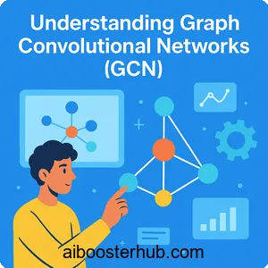
The power of graph convolutional networks lies in their ability to aggregate information from neighboring nodes, creating rich representations that capture both local structure and global patterns. This makes GCN particularly effective for tasks like semi-supervised classification, where we have limited labeled data but abundant structural information about how data points relate to each other.

Content

1. What are graph convolutional networks?

Graph convolutional networks represent a class of graph neural network (GNN) architectures that generalize the convolution operation from regular grids to arbitrary graph structures. To understand this concept, let’s first consider how traditional convolutional neural networks work on images.

In image processing, a convolutional filter slides across the pixel grid, computing weighted sums of neighboring pixels. The key insight is that nearby pixels are typically related, and this spatial relationship is captured through the convolution operation. But what happens when our data doesn’t lie on a regular grid? What if we’re dealing with social networks, molecular structures, or citation networks where connections are irregular?

This is where graph convolutional networks come in. A GCN extends the convolution concept to graphs by aggregating information from a node’s neighbors in the graph structure. Each node in the graph has features, and through successive GCN layers, nodes gather information from increasingly distant neighborhoods, building representations that encode both node features and graph topology.

The graph structure

Before diving deeper, let’s formalize what we mean by a graph. A graph ( G = (V, E) ) consists of:

A set of nodes (vertices) $ V = {v_1, v_2, …, v_n} $
A set of edges ( E ) connecting these nodes
A feature matrix $ X \in \mathbb{R}^{n \times d} $ where each row represents the features of a node
An adjacency matrix $ A \in \mathbb{R}^{n \times n} $ where $ A_{ij} = 1 $ if there’s an edge between nodes $ i $ and $ j $

For example, in a citation network, each paper is a node, citations are edges, and node features might include word embeddings from the paper’s abstract.

Core principles of GCN

The fundamental principle of graph convolutional networks is message passing. Each node sends messages to its neighbors, receives messages from them, and updates its representation based on this aggregated information. This process is repeated across multiple layers, allowing information to propagate through the graph structure.

Mathematically, a basic GCN layer can be expressed as:

$$ H^{(l+1)} = \sigma(\tilde{D}^{-\frac{1}{2}}\tilde{A}\tilde{D}^{-\frac{1}{2}}H^{(l)}W^{(l)}) $$

Where:

$ H^{(l)} $ is the matrix of node representations at layer ( l )
$ \tilde{A} = A + I $ is the adjacency matrix with added self-connections
$ \tilde{D} $ is the degree matrix of $ \tilde{A} $
$ W^{(l)} $ is the learnable weight matrix
$ \sigma $ is an activation function (e.g., ReLU)

2. The mathematical foundation: From spectral graph theory to GCN

The theoretical foundation of graph convolutional networks draws heavily from spectral graph theory, which studies graphs through the lens of linear algebra and eigenanalysis. While you don’t need to master spectral graph theory to use GCN effectively, understanding its origins provides valuable intuition.

Spectral convolutions on graphs

In spectral graph theory, we can define convolutions on graphs using the graph Laplacian matrix. The normalized graph Laplacian is defined as:

$$ L = I – D^{-\frac{1}{2}}AD^{-\frac{1}{2}} $$

Where $ D $ is the degree matrix. The Laplacian’s eigenvectors form a Fourier basis for the graph, allowing us to define convolution in the spectral domain. However, computing eigendecompositions is expensive for large graphs.

Simplification through localization

The breakthrough that led to practical GCN architectures came from localizing the spectral filters. Instead of working in the spectral domain, researchers developed approximations that operate directly on the graph structure. The key insight was to use Chebyshev polynomials to approximate spectral filters, and then further simplify by limiting to first-order approximations.

This simplification leads to the GCN propagation rule we saw earlier, which is computationally efficient and doesn’t require eigendecomposition. The symmetric normalization $ \tilde{D}^{-\frac{1}{2}}\tilde{A}\tilde{D}^{-\frac{1}{2}} $ ensures that the aggregation process is stable and doesn’t amplify node features unpredictably based on node degree.

Why normalization matters

Consider a node with many neighbors versus one with few. Without normalization, the node with many neighbors would accumulate much larger values during aggregation, leading to unstable training. The symmetric normalization effectively computes a weighted average where each neighbor’s contribution is scaled by the square root of both nodes’ degrees.

For a node $ i $ receiving information from neighbor $ j $, the normalization factor is:

$$ \frac{1}{\sqrt{deg(i)} \cdot \sqrt{deg(j)}} $$

This ensures that high-degree nodes don’t dominate the aggregation process.

3. GCN architecture and layer design

Now that we understand the mathematical foundation, let’s explore how to build practical graph convolutional networks. The gcn architecture typically consists of multiple stacked GCN layers, with each layer performing neighborhood aggregation followed by a non-linear transformation.

Basic GCN layer implementation

Here’s a simple implementation of a GCN layer in Python using PyTorch:

import torch
import torch.nn as nn
import torch.nn.functional as F

class GCNLayer(nn.Module):
    def __init__(self, in_features, out_features):
        super(GCNLayer, self).__init__()
        self.linear = nn.Linear(in_features, out_features)
    
    def forward(self, X, A_norm):
        """
        X: Node feature matrix (n_nodes, in_features)
        A_norm: Normalized adjacency matrix (n_nodes, n_nodes)
        """
        # Aggregate neighbor features
        aggregated = torch.mm(A_norm, X)
        # Apply linear transformation
        output = self.linear(aggregated)
        return output

def normalize_adjacency(A):
    """Compute D^(-1/2) * A * D^(-1/2)"""
    # Add self-connections
    A_tilde = A + torch.eye(A.size(0))
    # Compute degree matrix
    D_tilde = torch.diag(A_tilde.sum(dim=1))
    # Compute D^(-1/2)
    D_tilde_inv_sqrt = torch.diag(torch.pow(D_tilde.diag(), -0.5))
    # Compute normalized adjacency
    A_norm = torch.mm(torch.mm(D_tilde_inv_sqrt, A_tilde), D_tilde_inv_sqrt)
    return A_norm

Multi-layer GCN architecture

A complete GCN model typically stacks multiple layers with activation functions in between:

class GCN(nn.Module):
    def __init__(self, input_dim, hidden_dim, output_dim, dropout=0.5):
        super(GCN, self).__init__()
        self.gcn1 = GCNLayer(input_dim, hidden_dim)
        self.gcn2 = GCNLayer(hidden_dim, output_dim)
        self.dropout = dropout
    
    def forward(self, X, A_norm):
        # First GCN layer
        H = self.gcn1(X, A_norm)
        H = F.relu(H)
        H = F.dropout(H, self.dropout, training=self.training)
        
        # Second GCN layer
        output = self.gcn2(H, A_norm)
        return output

Design considerations

When designing a GCN architecture, several factors deserve attention:

Number of layers: Each GCN layer aggregates information from one-hop neighbors. A two-layer GCN captures information from two-hop neighborhoods, a three-layer GCN from three-hop neighborhoods, and so on. However, very deep GCN models can suffer from over-smoothing, where all node representations become too similar.

Hidden dimensions: Larger hidden dimensions provide more expressive power but increase computational cost and risk of overfitting, especially with limited labeled data.

Dropout: Regularization through dropout is crucial for GCN, particularly in semi-supervised settings where labeled data is scarce.

Activation functions: ReLU is commonly used, but alternatives like LeakyReLU or ELU can sometimes improve performance.

4. Semi-supervised classification with graph convolutional networks

One of the most powerful applications of graph convolutional networks is semi-supervised classification, where we leverage both limited labeled data and the graph structure to make predictions. This scenario is extremely common in real-world applications where labeling is expensive but relational information is abundant.

The semi-supervised learning paradigm

In semi-supervised classification with graph convolutional networks, we have:

A graph with $ n $ nodes
Feature vectors for all nodes
Labels for only a small subset of nodes (often less than 5% of the total)
The goal: predict labels for unlabeled nodes

The key insight is that connected nodes in the graph often share similar labels. For example, in a citation network, papers that cite each other often belong to the same research area. GCN exploits this structural information through message passing.

Training process

The training process for semi-supervised classification involves:

Forward pass: Propagate features through GCN layers for all nodes
Loss computation: Calculate loss only on labeled nodes
Backpropagation: Update weights to minimize loss
Inference: Use the trained model to predict labels for unlabeled nodes

Here’s a complete training example:

import torch.optim as optim

# Initialize model
input_dim = 128  # feature dimension
hidden_dim = 64
num_classes = 7
model = GCN(input_dim, hidden_dim, num_classes)

# Prepare data
X = torch.randn(2708, input_dim)  # Node features (e.g., Cora dataset)
A = torch.randint(0, 2, (2708, 2708)).float()  # Adjacency matrix
A = (A + A.t()) / 2  # Make symmetric
A_norm = normalize_adjacency(A)

labels = torch.randint(0, num_classes, (2708,))
train_mask = torch.zeros(2708, dtype=torch.bool)
train_mask[:140] = True  # Only 140 labeled nodes

# Training loop
optimizer = optim.Adam(model.parameters(), lr=0.01, weight_decay=5e-4)
model.train()

for epoch in range(200):
    optimizer.zero_grad()
    
    # Forward pass for all nodes
    output = model(X, A_norm)
    
    # Compute loss only on labeled nodes
    loss = F.cross_entropy(output[train_mask], labels[train_mask])
    
    # Backward pass
    loss.backward()
    optimizer.step()
    
    if epoch % 20 == 0:
        print(f'Epoch {epoch}, Loss: {loss.item():.4f}')

# Evaluation
model.eval()
with torch.no_grad():
    output = model(X, A_norm)
    predictions = output.argmax(dim=1)

Why GCN excels at semi-supervised learning

Graph convolutional networks are particularly effective for semi-supervised classification because:

Label propagation: Information from labeled nodes naturally propagates to their neighbors through the message passing mechanism. A node connected to multiple nodes of the same class will receive strong signals about its likely label.

Feature smoothing: GCN smooths features across connected nodes, creating consistent representations in densely connected regions. This reduces the impact of noisy features for individual nodes.

Transductive learning: The model sees all nodes during training (both labeled and unlabeled), allowing it to learn better representations by leveraging the full graph structure.

Real-world example: Document classification

Consider a citation network where each paper is a node and citations are edges. With GCN, we can classify papers into research topics using:

Node features: TF-IDF vectors or word embeddings from paper abstracts
Graph structure: Citation relationships
Labels: Research categories for a small subset of papers

A two-layer GCN can achieve impressive accuracy (often 80%+) even when only 5% of papers are labeled, because citations provide strong signals about topical similarity.

5. Advanced techniques and variants

While the basic GCN architecture is powerful, researchers have developed numerous extensions to address its limitations and expand its capabilities. Understanding these variants helps you choose the right approach for your specific problem.

Handling directed and weighted graphs

The standard GCN formulation assumes undirected, unweighted graphs. For directed graphs (like web links or social follows), you can:

Use the directed adjacency matrix directly
Symmetrize by adding transpose: $ A_{sym} = A + A^T $
Use separate weight matrices for incoming and outgoing edges

For weighted graphs (like knowledge graphs with different relation types), incorporate edge weights into the normalized adjacency matrix:

def normalize_weighted_adjacency(A_weighted):
    """Normalize weighted adjacency matrix"""
    A_tilde = A_weighted + torch.eye(A_weighted.size(0))
    D_tilde = torch.diag(A_tilde.sum(dim=1))
    D_tilde_inv_sqrt = torch.diag(torch.pow(D_tilde.diag(), -0.5))
    A_norm = torch.mm(torch.mm(D_tilde_inv_sqrt, A_tilde), D_tilde_inv_sqrt)
    return A_norm

Attention mechanisms: Graph Attention Networks

Graph Attention Networks (GAT) extend GCN by learning attention weights for different neighbors. Instead of treating all neighbors equally, GAT learns which neighbors are most important:

$$ \alpha_{ij} = \frac{\exp(\text{LeakyReLU}(a^T[Wh_i || Wh_j]))}{\sum_{k \in \mathcal{N}(i)} \exp(\text{LeakyReLU}(a^T[Wh_i || Wh_k]))} $$

Where $ \alpha_{ij} $ is the attention weight for neighbor $ j $ of node $ i $, and $ || $ denotes concatenation.

Sampling strategies for large graphs

For very large graphs (millions of nodes), computing full-batch GCN becomes impractical. Several sampling approaches have been developed:

GraphSAGE: Instead of using all neighbors, sample a fixed number of neighbors at each layer. This enables mini-batch training on large graphs.

FastGCN: Sample nodes per layer rather than per node, reducing computational complexity.

Cluster-GCN: Partition the graph into clusters and train on subgraphs, maintaining most connectivity within batches.

Addressing over-smoothing

Deep GCN models (many layers) can suffer from over-smoothing, where all node representations converge to similar values. Solutions include:

Residual connections: Add skip connections similar to ResNet: $$ H^{(l+1)} = \sigma(\tilde{D}^{-\frac{1}{2}}\tilde{A}\tilde{D}^{-\frac{1}{2}}H^{(l)}W^{(l)}) + H^{(l)} $$

Initial residual connections: Connect each layer directly to the input features to preserve original information.

DropEdge: Randomly drop edges during training to reduce over-smoothing and improve generalization.

6. Practical applications and use cases

Graph convolutional networks have found success across diverse domains where relational structure is important. Understanding these applications helps identify opportunities to apply GCN to your own problems.

Social network analysis

In social networks, GCN can predict user attributes, detect communities, or recommend connections. For example, predicting user interests based on:

Node features: Profile information, activity history
Graph structure: Friend connections, interactions
Task: Semi-supervised classification of user interests

Molecular property prediction

Drug discovery benefits enormously from GCN. Molecules are naturally represented as graphs (atoms as nodes, bonds as edges), and GCN can predict:

Toxicity
Solubility
Binding affinity
Drug-drug interactions

Each atom’s features might include atomic number, charge, and hybridization, while bonds provide the graph structure.

Knowledge graph completion

Knowledge graphs store facts as (subject, relation, object) triples. GCN helps predict missing links by learning entity and relation embeddings that capture the graph structure. This enables:

Answering complex queries
Reasoning about relationships
Discovering new connections

Recommendation systems

E-commerce and content platforms use GCN for recommendations by modeling user-item interactions as bipartite graphs:

Nodes: Users and items
Edges: Interactions (purchases, views, ratings)
Task: Predict which items a user might like

GCN captures both collaborative filtering signals (similar users like similar items) and content features.

Traffic prediction

Transportation networks naturally form graphs (intersections as nodes, roads as edges). GCN can predict traffic conditions by:

Aggregating information from nearby road segments
Incorporating temporal patterns with recurrent layers
Handling irregular network topology

Biological networks

Protein-protein interaction networks, brain connectivity graphs, and gene regulatory networks all benefit from GCN for:

Function prediction
Disease association
Network analysis

7. Implementation best practices and tips

Successfully implementing graph convolutional networks requires attention to several practical considerations that can significantly impact performance.

Data preprocessing

Feature normalization: Always normalize node features before training. Standard scaling or min-max normalization helps with gradient flow:

from sklearn.preprocessing import StandardScaler

scaler = StandardScaler()
X_normalized = scaler.fit_transform(X.numpy())
X = torch.FloatTensor(X_normalized)

Graph preprocessing: For very large graphs, consider:

Removing low-degree nodes that don’t contribute much information
Simplifying multi-graphs by aggregating multiple edges
Adding self-loops if not already present

Hyperparameter tuning

Critical hyperparameters for GCN include:

Learning rate: Start with 0.01 and use learning rate scheduling if needed. GCN training can be sensitive to learning rates.

Weight decay: Crucial for preventing overfitting in semi-supervised settings. Values between 5e-4 and 5e-3 often work well.

Dropout rate: Higher dropout (0.5-0.6) is often beneficial for GCN due to the semi-supervised nature.

Number of layers: Start with 2-3 layers. More layers don’t always help and can cause over-smoothing.

Handling class imbalance

In semi-supervised classification with graph convolutional networks, class imbalance in labeled data is common. Address this by:

Using weighted loss functions
Oversampling minority classes in the training mask
Adjusting decision thresholds during inference

Computational efficiency

For large graphs:

Precompute the normalized adjacency matrix
Use sparse matrix operations when possible
Consider sampling-based methods for graphs with millions of nodes
Leverage GPU acceleration for matrix multiplications

# Using sparse matrices for efficiency
import scipy.sparse as sp

def sparse_normalize_adjacency(A_sparse):
    """Normalize sparse adjacency matrix"""
    A_sparse = A_sparse + sp.eye(A_sparse.shape[0])
    rowsum = np.array(A_sparse.sum(1))
    d_inv_sqrt = np.power(rowsum, -0.5).flatten()
    d_inv_sqrt[np.isinf(d_inv_sqrt)] = 0.
    d_mat_inv_sqrt = sp.diags(d_inv_sqrt)
    return d_mat_inv_sqrt.dot(A_sparse).dot(d_mat_inv_sqrt)

Debugging and validation

Common issues and solutions:

NaN losses: Check for isolated nodes, ensure proper normalization, verify no division by zero in degree calculations.

Poor performance: Try simpler models first, verify graph structure is meaningful, ensure sufficient labeled examples per class.

Overfitting: Increase dropout, add weight decay, reduce model capacity, or add more regularization.

8. Conclusion

Graph convolutional networks represent a fundamental advancement in deep learning, extending neural networks to graph-structured data. By elegantly combining ideas from spectral graph theory with practical deep learning techniques, GCN enables powerful semi-supervised classification and representation learning on graphs. The architecture’s ability to aggregate neighborhood information through message passing makes it particularly effective when structural relationships contain valuable signals about node properties.

As graph neural network research continues to evolve, GCN remains a cornerstone architecture that every AI practitioner should understand. Whether you’re working with social networks, molecular structures, knowledge graphs, or recommendation systems, the principles and techniques covered in this article provide a solid foundation for applying graph convolutional networks to real-world problems. Start with the basic two-layer architecture, experiment with your specific graph data, and gradually explore more advanced variants as your needs grow.

Explore more:

Understanding Graph Convolutional Networks (GCN)