What Is Linear Regression? Complete Guide to Formula, Equation

Linear regression stands as one of the most fundamental and widely-used techniques in machine learning and statistical analysis. Whether you’re predicting house prices, forecasting sales, or analyzing scientific data, understanding linear regression is essential for anyone working with data and artificial intelligence. This comprehensive guide will walk you through everything you need to know about linear regression, from basic concepts to practical implementation.

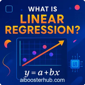
1. What is linear regression?

Linear regression is a statistical method used to model the relationship between a dependent variable (also called the target or output) and one or more independent variables (also called features or predictors) by fitting a linear equation to observed data. The linear regression meaning centers on finding the best-fitting straight line through your data points that minimizes the difference between predicted and actual values.

The Core Idea Behind Linear Regression

At its core, a linear regression model assumes that there’s a linear relationship between input variables and the output. This means that changes in the independent variables result in proportional changes in the dependent variable. The goal is to find the optimal parameters that define this relationship, allowing us to make predictions on new, unseen data.

An Intuitive Example of Linear Regression

The linear regression definition can be understood through a simple analogy: imagine you’re trying to predict how much ice cream a shop will sell based on the temperature outside. You collect data over several days and notice that as temperature increases, ice cream sales tend to increase as well. Linear regression helps you quantify this relationship with a mathematical equation that can predict sales for any given temperature.

Why linear regression matters in AI

Linear regression serves as a building block for understanding more complex machine learning algorithms. Many advanced techniques in AI, such as neural networks, can be viewed as extensions or generalizations of linear regression. Its simplicity makes it an excellent starting point for learning predictive modeling, while its interpretability makes it valuable in real-world applications where understanding the relationship between variables is crucial.

Key characteristics

• Interpretability: Linear regression models are highly interpretable, making it easy to understand how each input variable affects the output
• Efficiency: These models train quickly and require relatively little computational power
• Foundation: Understanding linear regression provides the groundwork for grasping more sophisticated machine learning techniques
• Versatility: Applicable across numerous domains, from economics to biology to engineering

2. Understanding the linear regression formula and equation

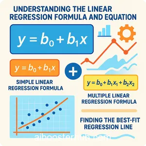
The mathematical foundation of linear regression is surprisingly elegant. Let’s break down the linear regression equation and understand each component.

Simple linear regression formula

For simple linear regression (with just one independent variable), the regression equation takes this form:

$$y = \beta_0 + \beta_1x + \epsilon$$

Where:

• \(y\) is the dependent variable (what we’re trying to predict)
• \(x\) is the independent variable (the feature we’re using to make predictions)
• \(\beta_0\) is the y-intercept (the value of \(y\) when \(x = 0\))
• \(\beta_1\) is the slope (how much \(y\) changes for each unit change in \(x\))
• \(\epsilon\) is the error term (the difference between predicted and actual values)

The regression line formula for predictions (without the error term) simplifies to:

$$\hat{y} = \beta_0 + \beta_1x$$

Here, \(\hat{y}\) (pronounced “y-hat”) represents the predicted value.

Multiple linear regression formula

When dealing with multiple independent variables, the linear formula extends naturally:

$$y = \beta_0 + \beta_1x_1 + \beta_2x_2 + … + \beta_nx_n + \epsilon$$

Or in matrix notation:

$$y = X\beta + \epsilon$$

Where \(X\) is the matrix of input features, and \(\beta\) is the vector of coefficients.

Finding the best-fit regression line

The key question is: how do we determine the optimal values for \(\beta_0\) and \(\beta_1\)? The answer lies in minimizing the sum of squared errors (SSE), also known as the residual sum of squares:

$$SSE = \sum_{i=1}^{n} (y_i – \hat{y}_i)^2 = \sum_{i=1}^{n} (y_i – (\beta_0 + \beta_1 x_i))^2$$

Using calculus, we can derive the closed-form solutions:

$$\beta_1 = \frac{\sum_{i=1}^{n}(x_i – \bar{x})(y_i – \bar{y})}{\sum_{i=1}^{n}(x_i – \bar{x})^2}$$

$$\beta_0 = \bar{y} – \beta_1\bar{x}$$

Where \(\bar{x}\) and \(\bar{y}\) are the means of \(x\) and \(y\) respectively.

3. Types of linear regression models

Linear regression comes in different flavors depending on the number of variables and the complexity of the relationship being modeled.

Simple linear regression

Simple linear regression involves one independent variable and one dependent variable. This is the most basic form of the linear regression model and is ideal for understanding fundamental concepts.

Linear regression example: Predicting a student’s final exam score based on the number of hours they studied.

import numpy as np
import matplotlib.pyplot as plt
from sklearn.linear_model import LinearRegression

# Sample data: hours studied vs exam score
hours_studied = np.array([1, 2, 3, 4, 5, 6, 7, 8]).reshape(-1, 1)
exam_scores = np.array([50, 55, 60, 65, 70, 75, 80, 85])

# Create and fit the model
model = LinearRegression()
model.fit(hours_studied, exam_scores)

# Get the regression line equation
slope = model.coef_[0]
intercept = model.intercept_

print(f"Regression equation: y = {intercept:.2f} + {slope:.2f}x")
print(f"If a student studies 5 hours: {model.predict([[5]])[0]:.2f} points")

# Visualize
plt.scatter(hours_studied, exam_scores, color='blue', label='Actual data')
plt.plot(hours_studied, model.predict(hours_studied), color='red', label='Regression line')
plt.xlabel('Hours Studied')
plt.ylabel('Exam Score')
plt.legend()
plt.title('Simple Linear Regression: Study Hours vs Exam Score')
plt.show()

Multiple linear regression

Multiple linear regression extends the simple linear regression model to include multiple independent variables. This allows for more complex and realistic modeling scenarios.

Example: Predicting house prices based on multiple features like square footage, number of bedrooms, age of the house, and location.

import pandas as pd
from sklearn.model_selection import train_test_split
from sklearn.linear_model import LinearRegression
from sklearn.metrics import mean_squared_error, r2_score

# Sample house data
data = {
    'square_feet': [1500, 1800, 2400, 2000, 2200, 1900, 2100, 2600],
    'bedrooms': [3, 3, 4, 3, 4, 3, 3, 4],
    'age': [10, 5, 15, 8, 3, 12, 7, 2],
    'price': [300000, 350000, 420000, 380000, 410000, 340000, 390000, 450000]
}

df = pd.DataFrame(data)

# Prepare features and target
X = df[['square_feet', 'bedrooms', 'age']]
y = df['price']

# Create and train model
model = LinearRegression()
model.fit(X, y)

# Display coefficients
print("Regression equation:")
print(f"Price = {model.intercept_:.2f}")
for feature, coef in zip(X.columns, model.coef_):
    print(f"  + {coef:.2f} × {feature}")

# Make a prediction
new_house = [[2000, 3, 5]]  # 2000 sq ft, 3 bedrooms, 5 years old
predicted_price = model.predict(new_house)[0]
print(f"\nPredicted price for new house: ${predicted_price:,.2f}")

Polynomial regression

While technically still a linear model (linear in the parameters), polynomial regression allows for curved relationships by adding polynomial terms of the features.

$$y = \beta_0 + \beta_1x + \beta_2x^2 + \beta_3x^3 + … + \epsilon$$

4. How linear regression works: The mechanics

Understanding what is a linear regression model requires grasping the underlying mechanism of how it learns from data.

The learning process

The linear fit process follows these steps:

1. Initialize parameters: Start with random or zero values for \(\beta_0\) and \(\beta_1\)
2. Make predictions: Use current parameter values to predict \(\hat{y}\) for all training samples
3. Calculate error: Compute the difference between predictions and actual values
4. Update parameters: Adjust parameters to minimize the error
5. Repeat: Continue until convergence or a maximum number of iterations

Ordinary least squares (OLS)

The most common method for finding the regression line equation parameters is Ordinary Least Squares. OLS minimizes the sum of squared residuals:

$$\min_{\beta_0, \beta_1} \sum_{i=1}^{n}(y_i – \beta_0 – \beta_1x_i)^2$$

The beauty of OLS is that it has a closed-form solution, meaning we can calculate the optimal parameters directly without iterative optimization.

Gradient descent alternative

For very large datasets or when closed-form solutions become computationally expensive, gradient descent offers an iterative approach:

import numpy as np

def gradient_descent_linear_regression(X, y, learning_rate=0.01, iterations=1000):
    """
    Implement linear regression using gradient descent
    """
    m = len(y)
    X_b = np.c_[np.ones((m, 1)), X]  # Add bias term
    theta = np.random.randn(X_b.shape[1], 1)  # Initialize parameters
    
    for iteration in range(iterations):
        # Calculate predictions
        predictions = X_b.dot(theta)
        
        # Calculate errors
        errors = predictions - y.reshape(-1, 1)
        
        # Calculate gradients
        gradients = (2/m) * X_b.T.dot(errors)
        
        # Update parameters
        theta = theta - learning_rate * gradients
        
        # Print progress every 100 iterations
        if iteration % 100 == 0:
            mse = np.mean(errors**2)
            print(f"Iteration {iteration}: MSE = {mse:.4f}")
    
    return theta

# Example usage
X = np.array([1, 2, 3, 4, 5])
y = np.array([2, 4, 5, 4, 5])

theta = gradient_descent_linear_regression(X, y)
print(f"\nFinal parameters: intercept = {theta[0][0]:.4f}, slope = {theta[1][0]:.4f}")

Assumptions of linear regression

For a linear regression model to produce reliable results, several assumptions must be satisfied:

1. Linearity: The relationship between independent and dependent variables is linear
2. Independence: Observations are independent of each other
3. Homoscedasticity: The variance of residuals is constant across all levels of independent variables
4. Normality: Residuals are normally distributed
5. No multicollinearity: Independent variables are not highly correlated with each other (for multiple regression)

5. Evaluating linear regression models

Once you’ve built a linear regression line, you need to assess how well it performs. Several metrics help evaluate model quality.

Coefficient of determination (R²)

R² measures the proportion of variance in the dependent variable explained by the independent variables:

$$R^2 = 1 – \frac{\sum_{i=1}^{n} (y_i – \hat{y}_i)^2}{\sum_{i=1}^{n} (y_i – \bar{y})^2}$$

R² ranges from 0 to 1, where:

• 0 means the model explains none of the variability
• 1 means the model explains all the variability
• Values closer to 1 indicate better fit

Mean squared error (MSE)

MSE measures the average squared difference between predicted and actual values:

$$MSE = \frac{1}{n}\sum_{i=1}^{n}(y_i – \hat{y}_i)^2$$

Lower MSE values indicate better model performance.

Root mean squared error (RMSE)

RMSE is simply the square root of MSE and has the same units as the target variable:

$$RMSE = \sqrt{MSE} = \sqrt{\frac{1}{n}\sum_{i=1}^{n}(y_i – \hat{y}_i)^2}$$

Mean absolute error (MAE)

MAE measures the average absolute difference between predictions and actual values:

$$MAE = \frac{1}{n}\sum_{i=1}^{n}|y_i – \hat{y}_i|$$

Practical evaluation example

from sklearn.model_selection import train_test_split
from sklearn.linear_model import LinearRegression
from sklearn.metrics import mean_squared_error, mean_absolute_error, r2_score
import numpy as np

# Generate sample data
np.random.seed(42)
X = np.random.rand(100, 1) * 10
y = 2.5 * X + 1.5 + np.random.randn(100, 1) * 2

# Split data
X_train, X_test, y_train, y_test = train_test_split(X, y, test_size=0.2, random_state=42)

# Train model
model = LinearRegression()
model.fit(X_train, y_train)

# Make predictions
y_pred_train = model.predict(X_train)
y_pred_test = model.predict(X_test)

# Evaluate
print("Training Set Performance:")
print(f"R² Score: {r2_score(y_train, y_pred_train):.4f}")
print(f"RMSE: {np.sqrt(mean_squared_error(y_train, y_pred_train)):.4f}")
print(f"MAE: {mean_absolute_error(y_train, y_pred_train):.4f}")

print("\nTest Set Performance:")
print(f"R² Score: {r2_score(y_test, y_pred_test):.4f}")
print(f"RMSE: {np.sqrt(mean_squared_error(y_test, y_pred_test)):.4f}")
print(f"MAE: {mean_absolute_error(y_test, y_pred_test):.4f}")

# Check for overfitting
if r2_score(y_train, y_pred_train) - r2_score(y_test, y_pred_test) > 0.1:
    print("\nWarning: Potential overfitting detected!")
else:
    print("\nModel generalizes well to test data.")

6. Real-world applications and examples

Linear regression finds applications across countless domains. Let’s explore several practical scenarios that demonstrate the versatility of this technique.

Sales forecasting

Businesses use linear regression to predict future sales based on factors like advertising spend, seasonality, and economic indicators.

import numpy as np
import pandas as pd
from sklearn.linear_model import LinearRegression
import matplotlib.pyplot as plt

# Sample marketing data
data = {
    'advertising_budget': [1000, 1500, 2000, 2500, 3000, 3500, 4000, 4500],
    'sales': [15000, 18000, 22000, 25000, 28000, 31000, 34000, 37000]
}

df = pd.DataFrame(data)

# Create and train model
X = df[['advertising_budget']]
y = df['sales']

model = LinearRegression()
model.fit(X, y)

# Predict sales for different budgets
future_budgets = np.array([[5000], [5500], [6000]])
predictions = model.predict(future_budgets)

print("Sales Predictions:")
for budget, sale in zip(future_budgets, predictions):
    print(f"  Budget: ${budget[0]:,} → Predicted Sales: ${sale:,.2f}")

print(f"\nFor every $1 increase in advertising, sales increase by ${model.coef_[0]:.2f}")

Healthcare and medicine

Medical researchers use linear regression to understand relationships between patient characteristics and health outcomes, such as predicting blood pressure based on age, weight, and lifestyle factors.

Real estate pricing

One of the most common applications is predicting property values based on features like location, size, amenities, and market conditions.

Climate science

Scientists use linear regression to analyze trends in temperature data, precipitation patterns, and other climate variables over time.

Financial analysis

Financial analysts employ regression models to understand relationships between stock prices and market indicators, predict returns, or assess risk factors.

Quality control in manufacturing

Manufacturers use linear regression to identify relationships between production parameters and product quality, enabling process optimization.

7. Advanced topics and considerations

As you advance in your understanding of what is a linear regression model, several important topics deserve attention.

Regularization techniques

When dealing with many features or potential overfitting, regularization helps by adding penalties to large coefficients:

Ridge Regression (L2 regularization): Adds squared magnitude of coefficients as penalty:

$$J(\beta) = \sum_{i=1}^{n} (y_i – \hat{y}_i)^2 + \lambda \sum_{j=1}^{p} \beta_j^2$$

Lasso Regression (L1 regularization): Adds absolute value of coefficients as penalty:

$$J(\beta) = \sum_{i=1}^{n} (y_i – \hat{y}_i)^2 + \lambda \sum_{j=1}^{p} |\beta_j|$$

from sklearn.linear_model import Ridge, Lasso
from sklearn.preprocessing import StandardScaler
import numpy as np

# Generate data with many features
np.random.seed(42)
X = np.random.randn(100, 20)
y = X[:, 0] * 3 + X[:, 1] * 2 + np.random.randn(100) * 0.5

# Standardize features
scaler = StandardScaler()
X_scaled = scaler.fit_transform(X)

# Compare regular, Ridge, and Lasso regression
from sklearn.linear_model import LinearRegression

models = {
    'Linear Regression': LinearRegression(),
    'Ridge Regression': Ridge(alpha=1.0),
    'Lasso Regression': Lasso(alpha=0.1)
}

for name, model in models.items():
    model.fit(X_scaled, y)
    print(f"\n{name}:")
    print(f"  Number of non-zero coefficients: {np.sum(model.coef_ != 0)}")
    print(f"  R² Score: {model.score(X_scaled, y):.4f}")

Feature engineering

Handling outliers

Outliers can significantly impact the regression line. Strategies include:

• Identifying outliers: Using residual plots or statistical tests
• Robust regression: Using methods less sensitive to outliers
• Transformation: Applying log or other transformations to reduce outlier impact
• Removal: Carefully removing extreme outliers after investigation

Cross-validation

To ensure your model generalizes well, use cross-validation:

from sklearn.model_selection import cross_val_score
from sklearn.linear_model import LinearRegression
import numpy as np

# Generate sample data
X = np.random.rand(100, 3)
y = X[:, 0] * 2 + X[:, 1] * 3 + X[:, 2] * 1.5 + np.random.randn(100) * 0.5

# Perform 5-fold cross-validation
model = LinearRegression()
scores = cross_val_score(model, X, y, cv=5, scoring='r2')

print("Cross-Validation R² Scores:", scores)
print(f"Mean R² Score: {scores.mean():.4f} (+/- {scores.std() * 2:.4f})")

When not to use linear regression

While powerful, linear regression isn’t always appropriate:

• Non-linear relationships: When the relationship between variables is inherently non-linear
• Classification problems: Use logistic regression or other classification algorithms instead
• Time series with strong autocorrelation: Consider ARIMA or other time series models
• High-dimensional data with complex interactions: Deep learning or tree-based methods may perform better

8. Conclusion

Linear regression remains one of the most important tools in the data scientist’s toolkit. From its elegant mathematical foundation expressed in the linear regression formula to its wide-ranging applications, understanding this technique provides both practical value and theoretical insight into more advanced machine learning methods.

The beauty of linear regression lies in its simplicity and interpretability—you can explain your model’s predictions in terms that non-technical stakeholders can understand. At the same time, it provides a springboard for understanding more complex algorithms in machine learning and artificial intelligence.