What is reinforcement learning: Basics to applications

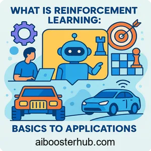
Reinforcement learning (RL) represents a unique approach to machine learning where agents learn to make decisions by interacting with their environment and receiving feedback through rewards or penalties. Unlike supervised learning, where models learn from labeled examples, or unsupervised learning, where patterns are discovered in unlabeled data, reinforcement learning focuses on learning optimal behavior through experience. This makes it particularly powerful for complex decision-making tasks, from playing chess to controlling autonomous vehicles.

Understanding RL basics requires exploring its roots in behavioral psychology, particularly operant conditioning and the work of B F Skinner. These foundations not only explain how organisms learn from consequences but also provide the theoretical framework for modern reinforcement learning algorithms. In this comprehensive reinforcement learning tutorial, we’ll explore the fundamentals of RL, examine both positive reinforcement and negative reinforcement, discuss reinforcement types and schedules, and demonstrate how these concepts translate into practical machine learning applications.

Content

1. Understanding reinforcement learning fundamentals

What is reinforcement learning in machine learning?

Reinforcement learning is a computational approach to learning from interaction. At its core, an RL system consists of an agent that takes actions in an environment, receives observations about the state of that environment, and obtains rewards based on its actions. The goal is to learn a policy—a strategy for selecting actions—that maximizes the cumulative reward over time.

The key components of any reinforcement learning system include:

Agent: The learner or decision-maker
Environment: Everything the agent interacts with
State: A representation of the current situation
Action: Choices available to the agent
Reward: Feedback signal indicating the desirability of an action
Policy: The agent’s strategy for selecting actions

What distinguishes reinforcement learning from other machine learning paradigms is the emphasis on sequential decision-making and delayed rewards. An agent must learn not just what action is best in a single moment, but how current actions affect future opportunities and rewards. This temporal aspect makes RL particularly suitable for problems involving planning, strategy, and long-term optimization.

The Markov decision process framework

The mathematical foundation of reinforcement learning is the Markov decision process (MDP). An MDP provides a formal framework for modeling decision-making situations where outcomes are partly random and partly under the control of the decision-maker. The Markov property states that the future state depends only on the current state and action, not on the sequence of events that preceded it.

Formally, an MDP is defined by the tuple $(S, A, P, R, \gamma)$, where:

$S$ is the set of possible states
$A$ is the set of possible actions
$P$ is the state transition probability function
$R$ is the reward function
$\gamma$ is the discount factor for future rewards

The agent’s objective is to find an optimal policy $\pi^*$ that maximizes the expected cumulative discounted reward:

$$ V^{\pi}(s) = \mathbb{E}\left[\sum_{t=0}^{\infty} \gamma^t R(s_t, a_t) \mid s_0 = s, \pi\right] $$

This value function represents the expected return when starting from state $s$ and following policy $\pi$. The optimal policy maximizes this value for all states, providing the foundation for various RL algorithms.

Reinforcement learning example: The grid world

To illustrate RL fundamentals, consider a simple grid world environment. An agent navigates a grid, trying to reach a goal state while avoiding obstacles. Each move incurs a small negative reward (cost), reaching the goal provides a large positive reward, and hitting obstacles results in penalties.

import numpy as np

class GridWorld:
    def __init__(self, size=5):
        self.size = size
        self.state = (0, 0)  # Start position
        self.goal = (size-1, size-1)  # Goal position
        self.obstacles = [(1, 1), (2, 2), (3, 1)]
        
    def reset(self):
        """Reset environment to initial state"""
        self.state = (0, 0)
        return self.state
    
    def step(self, action):
        """Execute action and return new state, reward, done flag"""
        # Actions: 0=up, 1=right, 2=down, 3=left
        moves = [(-1, 0), (0, 1), (1, 0), (0, -1)]
        new_state = (
            self.state[0] + moves[action][0],
            self.state[1] + moves[action][1]
        )
        
        # Check boundaries
        if (new_state[0] < 0 or new_state[0] >= self.size or
            new_state[1] < 0 or new_state[1] >= self.size):
            return self.state, -1, False  # Hit wall
        
        # Check obstacles
        if new_state in self.obstacles:
            return self.state, -5, False  # Hit obstacle
        
        # Update state
        self.state = new_state
        
        # Check goal
        if self.state == self.goal:
            return self.state, 10, True  # Reached goal
        
        return self.state, -0.1, False  # Normal move cost

# Example usage
env = GridWorld()
state = env.reset()
print(f"Initial state: {state}")

# Take random actions
for _ in range(5):
    action = np.random.randint(0, 4)
    state, reward, done = env.step(action)
    print(f"Action: {action}, State: {state}, Reward: {reward}")
    if done:
        break

This reinforcement learning basics with examples demonstrates how an agent interacts with an environment, receiving rewards that guide its learning toward optimal behavior.

2. Roots in behavioral psychology: Operant conditioning

B F Skinner and the foundations of learning theory

The theoretical underpinnings of reinforcement learning trace back to behavioral psychology, particularly the work of B F Skinner on operant conditioning. Skinner’s research demonstrated that behavior is shaped by its consequences—a principle that directly parallels how RL agents learn from rewards and penalties.

Operant conditioning Skinner studied involves learning through the consequences of voluntary behavior. Unlike classical conditioning, where responses are triggered by stimuli (as in Pavlov’s dogs), operant conditioning focuses on how organisms learn to perform or avoid certain behaviors based on what follows those behaviors. This framework provides valuable insights into reinforcement types and how different consequences affect learning.

Skinner identified several key concepts that remain relevant to understanding both human learning and artificial reinforcement learning:

Reinforcement: Any consequence that increases the likelihood of a behavior
Punishment: Any consequence that decreases the likelihood of a behavior
Extinction: The gradual weakening of a behavior when consequences cease
Discrimination: Learning to respond differently in different contexts
Generalization: Applying learned behaviors to similar situations

Positive reinforcement vs negative reinforcement

Understanding the distinction between positive reinforcement and negative reinforcement is crucial for grasping RL basics. These terms are often confused, so let’s clarify them precisely.

Positive reinforcement involves adding a desirable stimulus after a behavior, thereby increasing the likelihood of that behavior recurring. Positive reinforcement examples include:

Giving a dog a treat when it sits on command
Receiving praise for completing a task well
Earning points in a game for achieving objectives
Getting a bonus for meeting sales targets

In machine learning, positive reinforcement corresponds to giving the agent a positive reward for desirable actions. For instance, a robot learning to navigate might receive positive rewards for moving closer to its destination.

Negative reinforcement involves removing an aversive stimulus after a behavior, also increasing the likelihood of that behavior. This is not the same as punishment. Negative reinforcement examples include:

Taking aspirin to remove a headache (removing pain reinforces taking aspirin)
Buckling a seatbelt to stop the car’s beeping alarm
Studying to reduce anxiety about an upcoming exam
Cleaning your room to stop a parent’s nagging

A common misconception is that negative reinforcement means punishment, but actually, negative reinforcement vs punishment are opposite concepts. Negative reinforcement increases behavior by removing something unpleasant, while punishment decreases behavior by adding something unpleasant or removing something pleasant.

Reinforcement types and their effects

Beyond the positive vs negative reinforcement distinction, reinforcement theory identifies several types based on their effects on learning:

Primary reinforcers are naturally rewarding stimuli that satisfy biological needs (food, water, warmth). In RL systems, these correspond to terminal rewards that directly relate to the agent’s ultimate objective.

Secondary reinforcers (or conditioned reinforcers) gain their rewarding properties through association with primary reinforcers. Money is a classic example—it’s valuable because it can be exchanged for primary reinforcers. In RL, intermediate rewards that don’t directly achieve the goal but indicate progress serve as secondary reinforcers.

Immediate vs delayed reinforcement significantly affects learning speed. Immediate feedback allows faster learning, while delayed reinforcement requires the agent to maintain memory of past actions. This temporal credit assignment problem—determining which past actions led to current rewards—is one of the central challenges in reinforcement learning.

3. Reinforcement schedules and learning patterns

Understanding schedules of reinforcement

One of Skinner’s most influential discoveries was how the timing and frequency of reinforcement dramatically affect learning and behavior persistence. Schedules of reinforcement describe the rules for when and how often reinforcement is delivered following a behavior.

These schedules fall into two main categories:

Continuous reinforcement occurs when every instance of a behavior is reinforced. This produces rapid initial learning but also quick extinction when reinforcement stops. In RL systems, this is analogous to receiving reward signals after every action.

Partial reinforcement (or intermittent reinforcement) occurs when only some instances of a behavior are reinforced. Surprisingly, behaviors learned under partial reinforcement are more resistant to extinction—a phenomenon known as the partial reinforcement effect. This has important implications for designing reward structures in RL systems.

Fixed ratio and variable ratio schedules

Ratio schedules base reinforcement on the number of responses, creating different learning patterns.

Fixed ratio schedules provide reinforcement after a set number of responses. For example, a factory worker might be paid for every 10 items produced, or a coffee shop might offer a free drink after every 9 purchases. Fixed ratio schedules typically produce:

High response rates
Brief pauses after reinforcement
Predictable behavior patterns

In reinforcement learning, fixed ratio corresponds to providing rewards at regular intervals of successful actions.

Variable ratio schedules provide reinforcement after an unpredictable number of responses, averaging to a certain ratio. Slot machines use variable ratio schedules—you might win on the 3rd pull, then the 15th, then the 8th, averaging to a win every 10 pulls. This schedule produces:

Very high, steady response rates
Strong resistance to extinction
Persistent behavior even with infrequent reinforcement

Variable ratio schedules explain why gambling can be so compelling and why exploration strategies in RL that occasionally discover high rewards can be highly effective.

Fixed interval and variable interval schedules

Interval schedules base reinforcement on time elapsed since the last reinforcement.

Fixed interval schedules provide reinforcement for the first response after a set time period. Think of checking your mailbox once daily or studying intensely right before a scheduled exam. These schedules produce:

Increased response rate as the interval end approaches
“Scalloped” pattern in cumulative response graphs
Strategic timing of effort

Variable interval schedules provide reinforcement after unpredictable time periods. Checking email throughout the day (never knowing when a new message will arrive) follows a variable interval pattern. This schedule produces:

Steady, moderate response rates
Good resistance to extinction
Consistent behavior over time

import random

class ReinforcementSchedule:
    """Simulate different reinforcement schedules"""
    
    @staticmethod
    def fixed_ratio(responses, ratio=5):
        """Fixed ratio: reinforce every N responses"""
        return responses % ratio == 0
    
    @staticmethod
    def variable_ratio(responses, average_ratio=5):
        """Variable ratio: reinforce on average every N responses"""
        return random.random() < (1.0 / average_ratio)
    
    @staticmethod
    def fixed_interval(time_since_last, interval=10):
        """Fixed interval: reinforce after fixed time period"""
        return time_since_last >= interval
    
    @staticmethod
    def variable_interval(time_since_last, average_interval=10):
        """Variable interval: reinforce after variable time period"""
        threshold = 1.0 - np.exp(-time_since_last / average_interval)
        return random.random() < threshold

# Demonstration
schedule = ReinforcementSchedule()

# Fixed ratio example
print("Fixed Ratio (every 5 responses):")
for response in range(1, 21):
    if schedule.fixed_ratio(response, ratio=5):
        print(f"  Response {response}: REINFORCED")

# Variable ratio example
print("\nVariable Ratio (average every 5 responses):")
random.seed(42)
reinforcements = 0
for response in range(1, 21):
    if schedule.variable_ratio(response, average_ratio=5):
        reinforcements += 1
        print(f"  Response {response}: REINFORCED")
print(f"  Total reinforcements: {reinforcements}")

Understanding these schedules helps RL practitioners design reward structures that promote desired learning patterns and behavior persistence.

4. Implementing basic reinforcement learning algorithms

Q-learning: A fundamental RL algorithm

Q-learning is one of the most influential RL algorithms, representing a model-free approach to learning optimal policies. The algorithm learns a Q-function (Q(s, a)) that estimates the expected cumulative reward for taking action (a) in state (s) and following the optimal policy thereafter.

The Q-learning update rule is:

$$ Q(s_t, a_t) \leftarrow Q(s_t, a_t) + \alpha \left[r_{t+1} + \gamma \max_{a} Q(s_{t+1}, a) – Q(s_t, a_t)\right] $$

where:

$\alpha$ is the learning rate
$r_{t+1}$ is the immediate reward
$\gamma$ is the discount factor
$\max_{a} Q(s_{t+1}, a)$ is the maximum Q-value for the next state

This algorithm demonstrates how positive reinforcement (positive rewards) and negative reinforcement (negative rewards removed over time) guide the agent toward optimal behavior.

import numpy as np

class QLearningAgent:
    def __init__(self, n_states, n_actions, learning_rate=0.1, 
                 discount_factor=0.95, epsilon=0.1):
        self.q_table = np.zeros((n_states, n_actions))
        self.lr = learning_rate
        self.gamma = discount_factor
        self.epsilon = epsilon
        self.n_actions = n_actions
    
    def select_action(self, state):
        """Epsilon-greedy action selection"""
        if np.random.random() < self.epsilon:
            return np.random.randint(self.n_actions)  # Explore
        return np.argmax(self.q_table[state])  # Exploit
    
    def update(self, state, action, reward, next_state, done):
        """Q-learning update rule"""
        current_q = self.q_table[state, action]
        
        if done:
            target_q = reward
        else:
            max_next_q = np.max(self.q_table[next_state])
            target_q = reward + self.gamma * max_next_q
        
        # Update Q-value
        self.q_table[state, action] += self.lr * (target_q - current_q)
    
    def train(self, env, episodes=1000):
        """Train the agent"""
        rewards_history = []
        
        for episode in range(episodes):
            state = env.reset()
            total_reward = 0
            done = False
            
            while not done:
                action = self.select_action(state)
                next_state, reward, done = env.step(action)
                
                self.update(state, action, reward, next_state, done)
                
                state = next_state
                total_reward += reward
            
            rewards_history.append(total_reward)
            
            if (episode + 1) % 100 == 0:
                avg_reward = np.mean(rewards_history[-100:])
                print(f"Episode {episode + 1}, Average Reward: {avg_reward:.2f}")
        
        return rewards_history

# Example: Training on GridWorld
class SimpleGridWorld:
    def __init__(self):
        self.size = 4
        self.goal = 15  # Bottom-right corner
        self.state = 0
        
    def reset(self):
        self.state = 0
        return self.state
    
    def step(self, action):
        # Actions: 0=up, 1=right, 2=down, 3=left
        row, col = self.state // self.size, self.state % self.size
        
        if action == 0 and row > 0:
            row -= 1
        elif action == 1 and col < self.size - 1:
            col += 1
        elif action == 2 and row < self.size - 1:
            row += 1
        elif action == 3 and col > 0:
            col -= 1
        
        self.state = row * self.size + col
        
        if self.state == self.goal:
            return self.state, 10, True
        
        return self.state, -0.1, False

# Train the agent
env = SimpleGridWorld()
agent = QLearningAgent(n_states=16, n_actions=4, learning_rate=0.1,
                       discount_factor=0.95, epsilon=0.1)

print("Training Q-Learning Agent...")
rewards = agent.train(env, episodes=500)

# Display learned policy
print("\nLearned Q-Table (showing best action for each state):")
for i in range(16):
    best_action = np.argmax(agent.q_table[i])
    actions = ['↑', '→', '↓', '←']
    print(f"State {i:2d}: {actions[best_action]}", end="  ")
    if (i + 1) % 4 == 0:
        print()

Policy gradient methods

While Q-learning learns value functions, policy gradient methods directly optimize the policy. These methods are particularly useful for continuous action spaces and stochastic policies. The policy is parameterized by $\theta$, and we aim to maximize expected reward:

$$J(\theta) = \mathbb{E}_{\tau \sim \pi_\theta} \big[ R(\tau) \big] $$

The policy gradient theorem provides a way to compute gradients of this objective:

$$\nabla_\theta J(\theta) =
\mathbb{E}_{\tau \sim \pi_\theta} \left[
\sum_{t=0}^{T}
\nabla_\theta \log \pi_\theta(a_t \mid s_t) \, R_t
\right] $$

This approach connects to reinforcement theory by directly strengthening policies that lead to positive outcomes and weakening those that lead to negative outcomes.

import numpy as np

class PolicyGradientAgent:
    def __init__(self, n_states, n_actions, learning_rate=0.01):
        # Initialize policy parameters (simple linear model)
        self.theta = np.random.randn(n_states, n_actions) * 0.01
        self.lr = learning_rate
        
    def softmax_policy(self, state):
        """Compute action probabilities using softmax"""
        logits = self.theta[state]
        exp_logits = np.exp(logits - np.max(logits))  # Numerical stability
        return exp_logits / np.sum(exp_logits)
    
    def select_action(self, state):
        """Sample action from policy"""
        probs = self.softmax_policy(state)
        return np.random.choice(len(probs), p=probs)
    
    def update(self, states, actions, rewards):
        """Update policy using REINFORCE algorithm"""
        T = len(states)
        
        # Compute returns (cumulative rewards)
        returns = np.zeros(T)
        G = 0
        for t in reversed(range(T)):
            G = rewards[t] + 0.95 * G
            returns[t] = G
        
        # Normalize returns
        returns = (returns - np.mean(returns)) / (np.std(returns) + 1e-8)
        
        # Update policy parameters
        for t in range(T):
            state = states[t]
            action = actions[t]
            G = returns[t]
            
            # Compute gradient
            probs = self.softmax_policy(state)
            grad = np.zeros_like(probs)
            grad[action] = 1
            grad -= probs
            
            # Update theta
            self.theta[state] += self.lr * G * grad

# Example usage with GridWorld
env = SimpleGridWorld()
agent = PolicyGradientAgent(n_states=16, n_actions=4, learning_rate=0.01)

print("Training Policy Gradient Agent...")
for episode in range(500):
    states, actions, rewards = [], [], []
    state = env.reset()
    done = False
    
    while not done:
        action = agent.select_action(state)
        states.append(state)
        actions.append(action)
        
        next_state, reward, done = env.step(action)
        rewards.append(reward)
        state = next_state
    
    agent.update(states, actions, rewards)
    
    if (episode + 1) % 100 == 0:
        total_reward = sum(rewards)
        print(f"Episode {episode + 1}, Total Reward: {total_reward:.2f}")

5. Advanced concepts and modern applications

Deep reinforcement learning

Deep reinforcement learning combines RL algorithms with deep neural networks, enabling agents to handle high-dimensional state spaces like images or complex sensor data. The breakthrough came with Deep Q-Networks (DQN), which learned to play Atari games directly from pixels.

DQN uses a neural network to approximate the Q-function and employs two key innovations:

Experience replay stores transitions in a replay buffer and samples mini-batches for training. This breaks correlations between consecutive samples and improves data efficiency—analogous to how intermittent reinforcement can strengthen learning.

Target networks maintain a separate network for computing target Q-values, updated periodically. This stabilizes training by preventing the target from moving too quickly.

The DQN loss function is:

$$L(\theta) =
\mathbb{E}_{(s, a, r, s’) \sim D} \left[
\left(
r + \gamma \max_{a’} Q\bigl(s’, a’; \theta^- \bigr)
– Q\bigl(s, a; \theta \bigr)
\right)^2
\right]$$

where $\theta^-$ represents the target network parameters and $D$ is the replay buffer.

Multi-agent reinforcement learning

Multi-agent reinforcement learning extends RL to scenarios with multiple interacting agents. This introduces additional complexity as each agent’s optimal policy depends on other agents’ policies. Applications include:

Autonomous vehicle coordination
Robotic swarm control
Multi-player game AI
Economic market simulation

Agents can be cooperative (working toward shared goals), competitive (zero-sum games), or mixed (both cooperation and competition). The Nash equilibrium concept from game theory provides a solution concept for multi-agent systems.

Real-world applications

Reinforcement learning has achieved remarkable success across diverse domains:

Game playing: RL agents have mastered complex games including Go (AlphaGo), chess, StarCraft II, and Dota 2, often surpassing human expert performance. These successes demonstrate RL’s capability for strategic reasoning and long-term planning.

Robotics: RL enables robots to learn manipulation skills, locomotion, and complex tasks through trial and error. Positive reinforcement for successful grasps and negative reinforcement for collisions guide robots toward skilled behavior.

Autonomous systems: Self-driving cars use RL for decision-making in traffic, while drones learn flight control and navigation. The framework naturally handles the sequential decision-making inherent in these domains.

Resource management: RL optimizes data center cooling, reducing energy consumption significantly. It also improves scheduling, resource allocation, and supply chain management.

Healthcare: RL assists in personalized treatment planning, optimizing medication dosages, and developing clinical decision support systems. The ability to learn from delayed outcomes makes RL suitable for medical applications.

Finance: Trading strategies, portfolio management, and risk assessment benefit from RL’s ability to learn from market dynamics and adapt to changing conditions.

6. Challenges and future directions

Sample efficiency and exploration

One major challenge in reinforcement learning is sample efficiency—the number of interactions needed to learn effective policies. While humans can learn from just a few examples, RL agents often require millions of interactions. This relates to reinforcement schedules: finding the right balance between exploration (trying new actions) and exploitation (using known good actions) remains an active research area.

The exploration-exploitation trade-off mirrors the tension between variable ratio schedules (encouraging exploration through unpredictable rewards) and fixed ratio schedules (efficient exploitation of known strategies).

Reward engineering and shaping

Designing appropriate reward functions is crucial but challenging. Sparse rewards (only at task completion) make learning difficult, while dense rewards risk reward hacking—agents finding unintended ways to maximize rewards without achieving the true objective.

Reward shaping adds intermediate rewards to guide learning, similar to how secondary reinforcers in operant conditioning bridge the gap to primary goals. However, poorly designed shaping can introduce biases or create local optima.

Transfer learning and generalization

Current RL agents often struggle to transfer learned skills to new situations—a stark contrast to human adaptability. While classical conditioning and operant conditioning naturally exhibit generalization, RL systems require explicit mechanisms for transfer learning.

Meta-learning and few-shot learning approaches aim to develop agents that learn how to learn, acquiring skills that generalize across tasks with minimal additional training.

Safety and robustness

Deploying RL in real-world systems raises safety concerns. Agents might take dangerous exploratory actions or learn policies that work in training but fail catastrophically in slightly different conditions. Safe RL research focuses on:

Constraint satisfaction during learning
Robust policies that handle uncertainty
Interpretable decision-making
Learning from demonstrations to avoid dangerous exploration

Ethical considerations

As RL systems become more capable and autonomous, ethical questions arise. How do we encode human values into reward functions? How do we ensure fairness and prevent discrimination? These questions echo long-standing debates in behavioral psychology about the ethics of behavior modification through reinforcement.

7. Conclusion

Reinforcement learning represents a powerful framework for teaching agents to make decisions through interaction and feedback. From its roots in behavioral psychology and B F Skinner’s operant conditioning research to modern deep RL applications, the field has evolved dramatically while maintaining core principles about learning from consequences.

Understanding RL basics—including the distinction between positive reinforcement and negative reinforcement, the importance of reinforcement schedules, and the mathematical foundations in Markov decision processes—provides essential knowledge for anyone working with AI systems. The reinforcement learning examples and code implementations throughout this tutorial demonstrate how these concepts translate into practical algorithms that solve complex problems. As RL continues advancing toward more sample-efficient, generalizable, and safe systems, its applications will expand further, making it an increasingly vital tool in the AI practitioner’s toolkit.

Explore more: