Word Embeddings: Word2Vec, GloVe & Text Embedding Guide
Natural language processing has revolutionized how machines understand human language, and at the heart of this transformation lies a powerful concept: word embeddings. These numerical representations have become the foundation of modern AI systems, enabling computers to grasp the nuances of language in ways that were previously impossible. Whether you’re building a chatbot, analyzing sentiment, or creating a recommendation system, understanding word embeddings is essential for anyone working with text data.
Content
Toggle1. What are word embeddings?
The fundamental concept
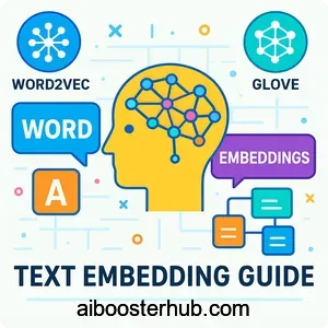
Word embeddings are dense vector representations of words that capture their semantic meaning and contextual relationships. Unlike traditional one-hot encoding, where each word is represented as a sparse vector with a single 1 and thousands of zeros, word embedding transforms words into continuous vectors in a lower-dimensional space. This approach allows machines to understand that “king” and “queen” are more related than “king” and “apple.”
The embedding meaning goes beyond simple word representation. Each dimension in these vectors captures different linguistic properties—some might encode gender, others might capture singular versus plural distinctions, and still others might represent abstract semantic concepts. This distributed representation enables powerful mathematical operations on words.
Why traditional methods fall short
Before word embeddings revolutionized NLP, researchers relied on methods like bag-of-words or TF-IDF (Term Frequency-Inverse Document Frequency). While these approaches could count word occurrences and measure importance, they fundamentally failed to capture semantic relationships. Two sentences with completely different words could express similar meanings, but traditional methods would see them as entirely unrelated.
Consider these sentences: “The dog runs quickly” and “The canine sprints rapidly.” A bag-of-words approach would find zero overlap, despite their semantic similarity. Word embeddings solve this by placing “dog” and “canine,” as well as “runs” and “sprints,” close together in vector space, enabling the model to recognize their similarity.
2. The evolution of word embeddings
From neural language models to Word2Vec
The journey toward modern embeddings began with neural language models that learned to predict words based on their context. However, it was Word2Vec, introduced by researchers at Google, that truly democratized word embeddings. Word2Vec offered two innovative architectures: Continuous Bag of Words (CBOW) and Skip-gram.
CBOW predicts a target word from its surrounding context words. If you have the sentence “The cat sat on the ___,” CBOW uses “The,” “cat,” “sat,” “on,” and “the” to predict “mat.” The Skip-gram model works in reverse—it predicts context words from a target word. Given “mat,” it tries to predict the surrounding words.
The Word2Vec training objective for Skip-gram can be expressed mathematically. For a sequence of training words \( w_1, w_2, …, w_T \), the objective is to maximize:
$$ \frac{1}{T} \sum_{t=1}^{T} \sum_{-c \leq j \leq c, j \neq 0} \log p(w_{t+j} | w_t) $$
where \( c \) is the context window size. The probability \( p(w_O | w_I) \) is calculated using softmax:
$$ p(w_O | w_I) = \frac{\exp(v_{w_O}^T v_{w_I})}{\sum_{w=1}^{W} \exp(v_w^T v_{w_I})} $$
Here’s a practical example using Python with the Gensim library:
from gensim.models import Word2Vec
import numpy as np

# Sample sentences for training
sentences = [
    ['the', 'cat', 'sits', 'on', 'the', 'mat'],
    ['the', 'dog', 'runs', 'in', 'the', 'park'],
    ['cats', 'and', 'dogs', 'are', 'pets'],
    ['the', 'quick', 'brown', 'fox', 'jumps'],
]

# Train Word2Vec model
model = Word2Vec(sentences, vector_size=100, window=5,
                 min_count=1, workers=4, sg=1)  # sg=1 for Skip-gram

# Get word embedding for 'cat'
cat_vector = model.wv['cat']
print(f"Embedding dimension: {len(cat_vector)}")

# Find similar words
similar_words = model.wv.most_similar('cat', topn=3)
print(f"Words similar to 'cat': {similar_words}")

# Vector arithmetic: king - man + woman ≈ queen
result = model.wv.most_similar(positive=['king', 'woman'],
                                negative=['man'], topn=1)
print(f"King - man + woman = {result}")
GloVe embedding: capturing global statistics
While Word2Vec focused on local context windows, GloVe (Global Vectors for Word Representation) took a different approach by incorporating global word co-occurrence statistics. GloVe constructs a word-word co-occurrence matrix from the entire corpus and factorizes it to produce word vectors.
The GloVe objective function combines the benefits of matrix factorization methods with the efficiency of local context window methods:
$$J = \sum_{i,j=1}^{V} f(X_{ij}) \, \big( w_i^{T} \tilde{w}_j + b_i + \tilde{b}_j – \log X_{ij} \big)^2$$
where \( X_{ij} \) represents the number of times word \( j \) appears in the context of word \( i \), \( w_i \) and \( \tilde{w}_j \) are word vectors, and \( f(X_{ij}) \) is a weighting function that prevents common word pairs from dominating the training.
3. How word embeddings capture meaning
Semantic similarity in vector space
One of the most remarkable properties of word embeddings is their ability to capture semantic similarity. Words with similar meanings end up close to each other in the embedding space. This proximity can be measured using cosine similarity:
$$ \text{similarity}(A, B) = \frac{A \cdot B}{||A|| \cdot ||B||} = \frac{\sum_{i=1}^{n} A_i B_i}{\sqrt{\sum_{i=1}^{n} A_i^2} \sqrt{\sum_{i=1}^{n} B_i^2}} $$
Values range from -1 (opposite meanings) to 1 (identical meanings), with 0 indicating no relationship.
Here’s how to calculate semantic similarity in practice:
from sklearn.metrics.pairwise import cosine_similarity
import numpy as np

# Example word vectors (simplified 5-dimensional)
king = np.array([0.5, 0.8, 0.3, 0.1, 0.9]).reshape(1, -1)
queen = np.array([0.6, 0.7, 0.4, 0.2, 0.8]).reshape(1, -1)
apple = np.array([0.1, 0.2, 0.9, 0.7, 0.1]).reshape(1, -1)

# Calculate similarities
king_queen_sim = cosine_similarity(king, queen)[0][0]
king_apple_sim = cosine_similarity(king, apple)[0][0]

print(f"Similarity between 'king' and 'queen': {king_queen_sim:.3f}")
print(f"Similarity between 'king' and 'apple': {king_apple_sim:.3f}")

# Using trained Word2Vec model
similarity = model.wv.similarity('cat', 'dog')
print(f"Word2Vec similarity between 'cat' and 'dog': {similarity:.3f}")
Analogical reasoning with word vectors
Perhaps the most famous demonstration of word embeddings’ power is their ability to solve analogies through vector arithmetic. The classic example is: “king” – “man” + “woman” ≈ “queen.” This works because embeddings capture relational semantics in the vector space geometry.
The analogy \( a:b :: c:d \) can be solved by finding the word \( d \) whose embedding is closest to:
$$ \vec{d} \approx \vec{b} – \vec{a} + \vec{c} $$
This property emerges from the training process and reveals that embeddings capture abstract relationships like gender, geography, and verb tense.
def solve_analogy(model, word1, word2, word3, topn=5):
    """
    Solve analogy: word1 is to word2 as word3 is to ?
    Example: king is to queen as man is to woman
    """
    try:
        result = model.wv.most_similar(
            positive=[word2, word3],
            negative=[word1],
            topn=topn
        )
        return result
    except KeyError as e:
        return f"Word not in vocabulary: {e}"

# Examples of analogies
print("Paris is to France as Berlin is to:")
print(solve_analogy(model, 'paris', 'france', 'berlin', topn=1))

print("\nWalk is to walked as go is to:")
print(solve_analogy(model, 'walk', 'walked', 'go', topn=1))
4. Text embedding and token embedding in modern NLP
Beyond single words: text embedding
While word embedding focuses on individual words, text embedding extends this concept to represent entire sentences, paragraphs, or documents as vectors. This is crucial for tasks like document classification, semantic search, and question answering where understanding the meaning of longer text sequences is essential.
Text embeddings can be created through various methods:
- Averaging word embeddings: Simply taking the mean of all word vectors in a sentence
- Weighted averaging: Using TF-IDF weights to emphasize important words
- Sentence encoders: Specialized models trained to create meaningful sentence-level representations
import numpy as np

def simple_text_embedding(sentence, model):
    """
    Create text embedding by averaging word embeddings
    """
    words = sentence.lower().split()
    word_vectors = []

    for word in words:
        if word in model.wv:
            word_vectors.append(model.wv[word])

    if word_vectors:
        # Average all word vectors
        text_embedding = np.mean(word_vectors, axis=0)
        return text_embedding
    return None

# Example usage
sentence1 = "the cat sits on the mat"
sentence2 = "a dog runs in the park"

embedding1 = simple_text_embedding(sentence1, model)
embedding2 = simple_text_embedding(sentence2, model)

if embedding1 is not None and embedding2 is not None:
    similarity = cosine_similarity(
        embedding1.reshape(1, -1),
        embedding2.reshape(1, -1)
    )[0][0]
    print(f"Sentence similarity: {similarity:.3f}")
Token embedding and the embedding layer
In neural network architectures, the embedding layer serves as the first layer that transforms discrete token IDs into dense vector representations. This layer is essentially a lookup table where each token has a corresponding embedding vector that gets updated during training.
The embedding layer performs a simple operation: given a token ID \( i \), it retrieves the \( i \)-th row from the embedding matrix \( E \in \mathbb{R}^{V \times d} \), where \( V \) is the vocabulary size and \( d \) is the embedding dimension.
Here’s how to implement an embedding layer in a neural network:
import torch
import torch.nn as nn

class SimpleTextClassifier(nn.Module):
    def __init__(self, vocab_size, embedding_dim, hidden_dim, output_dim):
        super(SimpleTextClassifier, self).__init__()

        # Embedding layer: converts token IDs to dense vectors
        self.embedding = nn.Embedding(vocab_size, embedding_dim)

        # Rest of the network
        self.fc1 = nn.Linear(embedding_dim, hidden_dim)
        self.fc2 = nn.Linear(hidden_dim, output_dim)
        self.relu = nn.ReLU()

    def forward(self, token_ids):
        # token_ids shape: (batch_size, sequence_length)
        embedded = self.embedding(token_ids)  # (batch_size, seq_len, embed_dim)

        # Pool embeddings by averaging across sequence length
        pooled = torch.mean(embedded, dim=1)  # (batch_size, embed_dim)

        # Pass through network
        hidden = self.relu(self.fc1(pooled))
        output = self.fc2(hidden)
        return output

# Example usage
vocab_size = 10000
embedding_dim = 128
hidden_dim = 64
output_dim = 2  # Binary classification

model = SimpleTextClassifier(vocab_size, embedding_dim, hidden_dim, output_dim)

# Sample input: batch of 2 sequences, each with 10 tokens
sample_input = torch.randint(0, vocab_size, (2, 10))
output = model(sample_input)

print(f"Input shape: {sample_input.shape}")
print(f"Output shape: {output.shape}")
print(f"Embedding layer weight shape: {model.embedding.weight.shape}")
Pre-trained embeddings versus learned embeddings
Modern NLP practitioners face a choice: use pre-trained embeddings or learn task-specific embeddings from scratch. Pre-trained embeddings like Word2Vec, GloVe, or FastText offer the advantage of capturing general language patterns learned from massive corpora. They’re particularly valuable when working with limited training data.
However, learned embeddings can be more effective for domain-specific tasks. For instance, medical text analysis might benefit from embeddings trained specifically on medical literature, capturing specialized terminology and relationships that general-purpose embeddings might miss.
# Loading pre-trained GloVe embeddings
def load_glove_embeddings(glove_file, embedding_dim):
    embeddings_index = {}
    with open(glove_file, 'r', encoding='utf-8') as f:
        for line in f:
            values = line.split()
            word = values[0]
            coefs = np.asarray(values[1:], dtype='float32')
            embeddings_index[word] = coefs
    return embeddings_index

# Create embedding matrix for your vocabulary
def create_embedding_matrix(vocab, embeddings_index, embedding_dim):
    embedding_matrix = np.zeros((len(vocab), embedding_dim))

    for i, word in enumerate(vocab):
        embedding_vector = embeddings_index.get(word)
        if embedding_vector is not None:
            embedding_matrix[i] = embedding_vector
        else:
            # Words not found will be initialized randomly
            embedding_matrix[i] = np.random.normal(0, 0.1, embedding_dim)

    return embedding_matrix

# Initialize PyTorch embedding layer with pre-trained weights
vocab = ['cat', 'dog', 'run', 'jump', 'happy']
embedding_dim = 100

# Assume we loaded GloVe embeddings
# embedding_matrix = create_embedding_matrix(vocab, glove_embeddings, 100)

# Create embedding layer with pre-trained weights
# embedding_layer = nn.Embedding.from_pretrained(
#     torch.FloatTensor(embedding_matrix),
#     freeze=False  # Set to True if you don't want to fine-tune
# )
5. Advanced concepts: contextual embeddings and transformers
The limitation of static embeddings
Traditional word embeddings like Word2Vec and GloVe have a significant limitation: they produce the same vector for a word regardless of context. The word “bank” receives identical representation whether referring to a financial institution or a river’s edge. This polysemy problem limits the expressiveness of static embeddings.
Consider these sentences:
- “I need to deposit money at the bank.”
- “We had a picnic on the river bank.”
Static embeddings cannot distinguish between these two meanings, treating “bank” identically in both contexts.
Contextual embeddings: ELMo, BERT, and beyond
Contextual embeddings revolutionized NLP by generating different vectors for the same word based on its surrounding context. Models like ELMo (Embeddings from Language Models) use bidirectional LSTMs to create context-aware representations, while BERT (Bidirectional Encoder Representations from Transformers) leverages the transformer architecture for even more powerful contextual understanding.
These models generate embeddings dynamically by processing the entire sentence, allowing “bank” to have different representations in different contexts. The embedding for each token is computed by considering all other tokens in the sequence through attention mechanisms.
from transformers import BertTokenizer, BertModel
import torch

# Load pre-trained BERT model and tokenizer
tokenizer = BertTokenizer.from_pretrained('bert-base-uncased')
model = BertModel.from_pretrained('bert-base-uncased')

def get_contextual_embedding(sentence):
    """
    Get contextual embeddings using BERT
    """
    # Tokenize and prepare input
    inputs = tokenizer(sentence, return_tensors='pt', padding=True)

    # Get embeddings
    with torch.no_grad():
        outputs = model(**inputs)

    # outputs.last_hidden_state shape: (batch_size, sequence_length, hidden_size)
    # Extract embeddings for each token
    token_embeddings = outputs.last_hidden_state

    return token_embeddings, inputs.tokens()

# Compare contextual embeddings for "bank" in different contexts
sentence1 = "I deposited money at the bank"
sentence2 = "We walked along the river bank"

embeddings1, tokens1 = get_contextual_embedding(sentence1)
embeddings2, tokens2 = get_contextual_embedding(sentence2)

print(f"Sentence 1 tokens: {tokens1}")
print(f"Sentence 2 tokens: {tokens2}")
print(f"Embedding shape for each sentence: {embeddings1.shape}")

# Find the token position of "bank" in each sentence and compare
# This would show different embeddings for "bank" in different contexts
Attention mechanisms and self-attention
At the core of modern contextual embeddings is the attention mechanism, particularly self-attention used in transformers. Self-attention allows each word to attend to all other words in the sequence, determining which words are most relevant for understanding its meaning.
The self-attention mechanism computes three vectors for each word: Query (Q), Key (K), and Value (V). The attention score is calculated as:
$$ \text{Attention}(Q, K, V) = \text{softmax}\left(\frac{QK^T}{\sqrt{d_k}}\right)V $$
where \( d_k \) is the dimension of the key vectors. This formula allows the model to create weighted combinations of all word embeddings, with weights determined by the relevance of each word to every other word.
6. Practical applications and best practices
Choosing the right embedding approach
Selecting the appropriate embedding method depends on your specific use case, dataset size, and computational resources. For simple classification tasks with limited data, starting with pre-trained Word2Vec or GloVe embeddings often provides good results with minimal computational overhead.
For more complex tasks requiring nuanced understanding of context—such as question answering, named entity recognition, or sentiment analysis—contextual embeddings from transformer models typically deliver superior performance. However, they come with increased computational costs and longer training times.
Consider these factors when choosing:
- Dataset size: Small datasets benefit from pre-trained embeddings
- Domain specificity: Specialized domains may need custom-trained embeddings
- Context importance: Tasks requiring disambiguation need contextual embeddings
- Computational budget: Static embeddings are much faster to use
- Multilingual needs: Models like multilingual BERT handle multiple languages
Fine-tuning and domain adaptation
Even when using pre-trained embeddings, fine-tuning them on your specific dataset can significantly improve performance. This process allows the model to adapt general language knowledge to your particular domain while maintaining the benefits of pre-training.
import torch.optim as optim

class DomainSpecificClassifier(nn.Module):
    def __init__(self, vocab_size, embedding_dim, hidden_dim, output_dim,
                 pretrained_embeddings=None):
        super(DomainSpecificClassifier, self).__init__()

        if pretrained_embeddings is not None:
            self.embedding = nn.Embedding.from_pretrained(
                pretrained_embeddings,
                freeze=False  # Allow fine-tuning
            )
        else:
            self.embedding = nn.Embedding(vocab_size, embedding_dim)

        self.lstm = nn.LSTM(embedding_dim, hidden_dim, batch_first=True)
        self.fc = nn.Linear(hidden_dim, output_dim)

    def forward(self, x):
        embedded = self.embedding(x)
        lstm_out, (hidden, cell) = self.lstm(embedded)
        # Use the last hidden state for classification
        output = self.fc(hidden[-1])
        return output

# Training loop with fine-tuning
def train_with_embeddings(model, train_loader, epochs, learning_rate):
    criterion = nn.CrossEntropyLoss()
    optimizer = optim.Adam(model.parameters(), lr=learning_rate)

    for epoch in range(epochs):
        model.train()
        total_loss = 0

        for batch_inputs, batch_labels in train_loader:
            optimizer.zero_grad()

            # Forward pass
            outputs = model(batch_inputs)
            loss = criterion(outputs, batch_labels)

            # Backward pass and optimization
            loss.backward()  # This updates embedding weights too
            optimizer.step()

            total_loss += loss.item()

        print(f"Epoch {epoch+1}/{epochs}, Loss: {total_loss/len(train_loader):.4f}")

# The embedding layer weights will be updated during training,
# adapting the pre-trained embeddings to your specific task
Handling out-of-vocabulary words
A common challenge with word embeddings is handling words that weren’t present in the training corpus. Several strategies address this:
Subword embeddings: Models like FastText represent words as bags of character n-grams, allowing them to generate embeddings for unknown words by combining subword information.
Special tokens: Using a special <UNK> token to represent all unknown words, though this loses information about the specific unknown word.
Character-level models: Building embeddings from character sequences, which can handle any word but may be computationally expensive.
# FastText example - handles out-of-vocabulary words
from gensim.models import FastText

# Train FastText model with character n-grams
sentences = [['the', 'cat', 'sits'], ['the', 'dog', 'runs']]
fasttext_model = FastText(sentences, vector_size=100, window=5,
                          min_count=1, workers=4, min_n=3, max_n=6)

# FastText can generate embeddings for words not in training
# It uses character n-grams to construct the embedding
oov_word = 'kittens'  # Not in training set
if oov_word not in fasttext_model.wv:
    # FastText can still generate an embedding
    oov_embedding = fasttext_model.wv[oov_word]
    print(f"Generated embedding for out-of-vocabulary word '{oov_word}'")
    print(f"Embedding shape: {oov_embedding.shape}")
Evaluation and visualization
Understanding the quality of your embeddings is crucial for debugging and improvement. Beyond task-specific metrics, intrinsic evaluation methods help assess embedding quality:
Analogy tasks: Testing whether embeddings can solve word analogies accurately measures their ability to capture semantic relationships.
Similarity benchmarks: Comparing embedding-based similarity scores with human judgments of word similarity.
Visualization: Reducing high-dimensional embeddings to 2D or 3D using techniques like t-SNE or UMAP helps visualize semantic clusters.
from sklearn.manifold import TSNE
import matplotlib.pyplot as plt

def visualize_embeddings(model, words, perplexity=5):
    """
    Visualize word embeddings in 2D using t-SNE
    """
    # Get embeddings for specified words
    word_vectors = []
    valid_words = []

    for word in words:
        if word in model.wv:
            word_vectors.append(model.wv[word])
            valid_words.append(word)

    # Reduce to 2D using t-SNE
    tsne = TSNE(n_components=2, perplexity=perplexity, random_state=42)
    embeddings_2d = tsne.fit_transform(word_vectors)

    # Plot
    plt.figure(figsize=(12, 8))
    plt.scatter(embeddings_2d[:, 0], embeddings_2d[:, 1], alpha=0.7)

    for i, word in enumerate(valid_words):
        plt.annotate(word, (embeddings_2d[i, 0], embeddings_2d[i, 1]),
                    fontsize=12, alpha=0.8)

    plt.title('Word Embedding Visualization using t-SNE')
    plt.xlabel('Dimension 1')
    plt.ylabel('Dimension 2')
    plt.grid(True, alpha=0.3)
    plt.tight_layout()
    return plt

# Visualize related words
animal_words = ['cat', 'dog', 'bird', 'fish', 'horse', 'lion']
action_words = ['run', 'jump', 'walk', 'swim', 'fly']
words_to_visualize = animal_words + action_words

# plot = visualize_embeddings(model, words_to_visualize)
# plt.show()
7. Conclusion
Word embeddings have fundamentally transformed how machines process and understand human language. From the foundational concepts of Word2Vec and GloVe embedding to the sophisticated contextual representations of modern transformer models, these vector representations enable AI systems to capture the rich semantic relationships inherent in language. Whether you’re working with simple token embedding in a classification task or implementing complex text embedding systems for semantic search, understanding these principles is essential for building effective NLP applications.
As you implement embeddings in your projects, remember that the choice between static and contextual embeddings, pre-trained and learned representations, depends heavily on your specific requirements. Start with simpler approaches when appropriate, and scale to more complex models as your needs demand. The field continues to evolve rapidly, but the fundamental insight remains powerful: by representing words as vectors in a learned semantic space, we enable machines to reason about language in increasingly human-like ways.
8. Knowledge Check
Quiz 1: Core Concepts of Word Embeddings
Quiz 2: Word2Vec Architectures
Quiz 3: The GloVe Model’s Approach
Quiz 4: Measuring Semantic Similarity
Quiz 5: Analogical Reasoning
king – man. Adding this difference vector to ‘woman’ results in a vector that is geometrically very close to the vector for ‘queen’.
