YOLO Object Detection: From YOLOv1 to YOLOv8
Object detection is one of the most fundamental tasks in computer vision, enabling machines to identify and locate objects within images or video streams. Among the various object detection algorithms available today, YOLO (You Only Look Once) stands out as a revolutionary approach that transformed the field by introducing real-time object detection capabilities. This comprehensive guide explores the YOLO algorithm, its evolution from YOLOv1 to YOLOv8, and why it has become the go-to solution for countless applications requiring fast and accurate object detection.
1. Understanding the YOLO algorithm
What makes YOLO different?
The YOLO algorithm introduced a paradigm shift in how machines detect objects. Unlike traditional object detection methods that apply a classifier to different regions of an image multiple times, YOLO treats object detection as a single regression problem. The name “You Only Look Once” perfectly captures this approach – the algorithm processes the entire image in one forward pass through a neural network, simultaneously predicting bounding boxes and class probabilities.
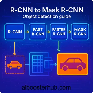
Traditional methods like R-CNN and its variants use a region proposal approach. They first generate potential bounding boxes where objects might be, then classify each region separately. This multi-stage pipeline is computationally expensive and slow. YOLO, on the other hand, divides the input image into a grid and predicts bounding boxes and class probabilities for each grid cell in a single evaluation.
The core concept
At its heart, the YOLO model works by dividing an input image into an \( S \times S \) grid. Each grid cell is responsible for detecting objects whose center falls within that cell. For each grid cell, the network predicts ( B ) bounding boxes along with confidence scores and ( C ) class probabilities.
The confidence score reflects how confident the model is that a box contains an object and how accurate the predicted box is. Mathematically, this is defined as:
$$ \text{Confidence} = Pr(\text{Object}) \times IOU_{\text{pred}}^{\text{truth}} $$
Where \( Pr(\text{Object}) \) is the probability that the cell contains an object, and \( IOU_{\text{pred}}^{\text{truth}} \) is the Intersection over Union between the predicted box and the ground truth.
Each bounding box consists of five predictions: ( x, y, w, h ), and confidence. The coordinates \( (x, y) \) represent the center of the box relative to the grid cell, while ( w ) and ( h ) represent the width and height relative to the whole image.
Why real-time object detection matters
Real-time object detection has opened doors to applications that were previously impossible or impractical. Autonomous vehicles need to detect pedestrians, other vehicles, and obstacles in milliseconds to make safe driving decisions. Surveillance systems must identify suspicious activities as they happen. Augmented reality applications require instant object recognition to overlay digital information on the physical world.
The YOLO algorithm made these applications feasible by achieving processing speeds of 45 frames per second or higher, while maintaining competitive accuracy with slower methods. This balance between speed and accuracy is what made YOLO so revolutionary and widely adopted.
2. YOLOv1: The revolutionary beginning
Architecture and innovation
YOLOv1, introduced in a groundbreaking paper, consisted of 24 convolutional layers followed by 2 fully connected layers. The architecture drew inspiration from the GoogLeNet model for image classification but was adapted for the detection task.
The network takes an input image of size \( 448 \times 448 \) pixels and outputs a tensor of size \( S \times S \times (B \times 5 + C) \), where ( S = 7 ), ( B = 2 ), and ( C = 20 ) for the PASCAL VOC dataset. This means the image is divided into a \( 7 \times 7 \) grid, with each cell predicting 2 bounding boxes and probabilities for 20 classes.
Loss function
YOLOv1 uses a multi-part loss function that penalizes localization errors, confidence errors, and classification errors. The loss function is:
$$\begin{aligned}
\mathcal{L} = \,
& \lambda_{\text{coord}} \sum_{i=0}^{S^2} \sum_{j=0}^{B}
\mathbb{1}_{ij}^{\text{obj}} \left[
(x_i – \hat{x}_i)^2 + (y_i – \hat{y}_i)^2
\right] \\
& + \lambda_{\text{coord}} \sum_{i=0}^{S^2} \sum_{j=0}^{B}
\mathbb{1}_{ij}^{\text{obj}} \left[
(\sqrt{w_i} – \sqrt{\hat{w}_i})^2 + (\sqrt{h_i} – \sqrt{\hat{h}_i})^2
\right] \\
& + \sum_{i=0}^{S^2} \sum_{j=0}^{B}
\mathbb{1}_{ij}^{\text{obj}} (C_i – \hat{C}_i)^2 \\
& + \lambda_{\text{noobj}} \sum_{i=0}^{S^2} \sum_{j=0}^{B}
\mathbb{1}_{ij}^{\text{noobj}} (C_i – \hat{C}_i)^2 \\
& + \sum_{i=0}^{S^2} \mathbb{1}_{i}^{\text{obj}}
\sum_{c \in \text{classes}} (p_i(c) – \hat{p}_i(c))^2
\end{aligned} $$
Where \( \mathbb{1}{ij}^{\text{obj}} \) indicates if object appears in cell ( i ) and predictor ( j ) is responsible for that prediction, and \( \lambda{\text{coord}} = 5 \) and \( \lambda_{\text{noobj}} = 0.5 \) are weights to balance the different components.
Limitations
Despite its innovation, YOLOv1 had notable limitations. It struggled with small objects, especially those appearing in groups, because each grid cell could only predict two boxes and belong to one class. The coarse grid structure (7×7) meant that nearby objects were difficult to detect separately. Additionally, the model had difficulty with objects in unusual aspect ratios since it learned from the training data distribution.
Simple implementation example
Here’s a simplified example of how to structure predictions in YOLO:
import numpy as np

def process_yolo_output(output, grid_size=7, num_boxes=2, num_classes=20):
    """
    Process YOLO output tensor

    Args:
        output: Network output of shape (grid_size, grid_size, num_boxes*5 + num_classes)
        grid_size: Grid dimension (S)
        num_boxes: Number of bounding boxes per cell (B)
        num_classes: Number of object classes (C)

    Returns:
        List of detected objects with [class, confidence, x, y, w, h]
    """
    detections = []

    for i in range(grid_size):
        for j in range(grid_size):
            cell_data = output[i, j, :]

            # Extract class probabilities
            class_probs = cell_data[num_boxes*5:]

            # Extract bounding boxes
            for b in range(num_boxes):
                box_data = cell_data[b*5:(b+1)*5]
                x, y, w, h, confidence = box_data

                # Convert relative coordinates to absolute
                x_abs = (j + x) / grid_size
                y_abs = (i + y) / grid_size

                # Calculate class-specific confidence
                class_confidences = confidence * class_probs
                best_class = np.argmax(class_confidences)
                best_confidence = class_confidences[best_class]

                if best_confidence > 0.5:  # Threshold
                    detections.append([
                        best_class, best_confidence,
                        x_abs, y_abs, w, h
                    ])

    return detections

# Example usage
output = np.random.rand(7, 7, 30)  # Simulated output
detections = process_yolo_output(output)
print(f"Found {len(detections)} objects")
3. Evolution through YOLOv2 and YOLOv3
Improvements
YOLOv2 (also called YOLO9000 for its ability to detect 9000+ object categories) addressed many of YOLOv1’s shortcomings. Key improvements included:
Batch Normalization: Adding batch normalization to all convolutional layers improved convergence and acted as a regularizer, eliminating the need for dropout. This single change improved mAP by 2%.
High-resolution classifier: YOLOv1 trained the classifier on \( 224 \times 224 \) images then switched to \( 448 \times 448 \) for detection. YOLOv2 first fine-tuned the classification network at \( 448 \times 448 \) for 10 epochs before doing detection, giving the network time to adjust to higher resolution input.
Anchor boxes: Instead of predicting coordinates directly, YOLOv2 predicted offsets from predetermined anchor boxes. This made the network easier to learn and improved recall. The network predicts 5 anchor boxes per grid cell, compared to YOLOv1’s 2 boxes.
Dimension clusters: Rather than hand-picking anchor box dimensions, YOLOv2 used k-means clustering on the training set bounding boxes to automatically find good priors.
Fine-grained features: YOLOv2 added a passthrough layer that brings high-resolution features from earlier in the network to help detect small objects. This concatenates higher resolution features with low resolution features, similar to ResNet skip connections.
YOLOv3: Multi-scale predictions
YOLOv3 made predictions at three different scales, dramatically improving detection of objects at different sizes. The network makes predictions at scales of 13×13, 26×26, and 52×52, using features from different depths of the network.
Feature Pyramid Network: YOLOv3 adopted ideas from Feature Pyramid Networks (FPN). Features are extracted from the backbone network at three different scales and used for prediction. This architecture allows the network to detect:
- Small objects in the 52×52 feature map
- Medium objects in the 26×26 feature map
- Large objects in the 13×13 feature map
Darknet-53 backbone: YOLOv3 uses a deeper feature extractor called Darknet-53, which has 53 convolutional layers. This backbone uses residual connections, making it more powerful while remaining efficient.
Multi-label classification: Instead of using softmax for class predictions (which assumes classes are mutually exclusive), YOLOv3 uses independent logistic classifiers. This allows the model to better handle datasets with overlapping labels.
Implementation of anchor boxes
Here’s how anchor boxes work in practice:
import numpy as np

def decode_yolo_boxes(predictions, anchors, grid_size, image_size):
    """
    Decode YOLO predictions with anchor boxes

    Args:
        predictions: Model output [batch, grid, grid, num_anchors, 5+num_classes]
        anchors: List of anchor box dimensions [(w1,h1), (w2,h2), ...]
        grid_size: Size of prediction grid
        image_size: Original image dimensions

    Returns:
        Decoded bounding boxes
    """
    num_anchors = len(anchors)
    batch_size = predictions.shape[0]

    # Create offset grid
    grid_x = np.arange(grid_size)
    grid_y = np.arange(grid_size)
    x_offset, y_offset = np.meshgrid(grid_x, grid_y)

    x_offset = np.reshape(x_offset, (1, grid_size, grid_size, 1))
    y_offset = np.reshape(y_offset, (1, grid_size, grid_size, 1))

    # Extract predictions
    box_xy = predictions[..., 0:2]  # Center x, y
    box_wh = predictions[..., 2:4]  # Width, height
    box_confidence = predictions[..., 4:5]
    box_class_probs = predictions[..., 5:]

    # Apply sigmoid to x, y coordinates and objectness
    box_xy = 1 / (1 + np.exp(-box_xy))
    box_confidence = 1 / (1 + np.exp(-box_confidence))

    # Adjust predictions to grid
    box_xy[..., 0] = (box_xy[..., 0] + x_offset) / grid_size
    box_xy[..., 1] = (box_xy[..., 1] + y_offset) / grid_size

    # Apply anchor boxes to width and height
    anchors_tensor = np.reshape(anchors, (1, 1, 1, num_anchors, 2))
    box_wh = np.exp(box_wh) * anchors_tensor / image_size

    # Convert to corner coordinates
    box_mins = box_xy - (box_wh / 2.)
    box_maxes = box_xy + (box_wh / 2.)

    boxes = np.concatenate([
        box_mins[..., 1:2],  # y_min
        box_mins[..., 0:1],  # x_min
        box_maxes[..., 1:2],  # y_max
        box_maxes[..., 0:1]   # x_max
    ], axis=-1)

    return boxes, box_confidence, box_class_probs

# Example usage
predictions = np.random.randn(1, 13, 13, 3, 85)  # 80 classes + 5
anchors = [(10,13), (16,30), (33,23)]
boxes, conf, probs = decode_yolo_boxes(predictions, anchors, 13, 416)
4. YOLOv4 and YOLOv5: The modern era
Innovations
YOLOv4 represented a major step forward by incorporating numerous techniques from recent research. The paper famously called these “Bag of Freebies” (improvements that increase accuracy without affecting inference speed) and “Bag of Specials” (improvements that slightly increase inference cost but significantly boost accuracy).
CSPDarknet53 backbone: YOLOv4 uses Cross Stage Partial connections (CSP) in the backbone network, which reduces computation while maintaining accuracy. CSP separates the feature map into two parts, only one of which passes through the dense block, reducing redundant gradient information.
Spatial Pyramid Pooling (SPP): An SPP layer is added to increase the receptive field and separate the most significant context features without reducing the network speed.
Path Aggregation Network (PANet): YOLOv4 uses PANet for the neck instead of Feature Pyramid Networks, improving information flow and feature fusion.
Mosaic data augmentation: This technique combines four training images into one, allowing the model to learn from a more diverse set of object scales and contexts in each batch.
YOLOv5: Practical implementation
YOLOv5, while controversial in its versioning (some argue it should have been called something else), became hugely popular due to its user-friendly PyTorch implementation and excellent documentation. It introduced several practical improvements:
Auto-learning anchor boxes: The model can automatically learn optimal anchor boxes for your dataset during training.
Model scaling: YOLOv5 comes in five variants (n, s, m, l, x) that scale both depth and width, making it easy to choose the right speed-accuracy tradeoff for your application.
Focus structure: A new Focus layer slices the input image into patches and concatenates them, reducing computation while maintaining information.
Here’s a practical example of using YOLOv5:
import torch
import cv2
import numpy as np

# Note: This requires YOLOv5 to be installed
# pip install yolov5

def run_yolov5_inference(image_path, conf_threshold=0.25):
    """
    Run inference using YOLOv5

    Args:
        image_path: Path to input image
        conf_threshold: Confidence threshold for detections

    Returns:
        Annotated image and detection results
    """
    # Load model
    model = torch.hub.load('ultralytics/yolov5', 'yolov5s', pretrained=True)
    model.conf = conf_threshold  # Set confidence threshold

    # Read image
    img = cv2.imread(image_path)
    img_rgb = cv2.cvtColor(img, cv2.COLOR_BGR2RGB)

    # Inference
    results = model(img_rgb)

    # Parse results
    detections = results.pandas().xyxy[0]  # Get detections as pandas DataFrame

    # Draw bounding boxes
    for idx, detection in detections.iterrows():
        x1, y1 = int(detection['xmin']), int(detection['ymin'])
        x2, y2 = int(detection['xmax']), int(detection['ymax'])
        conf = detection['confidence']
        cls = detection['name']

        # Draw rectangle
        cv2.rectangle(img, (x1, y1), (x2, y2), (0, 255, 0), 2)

        # Add label
        label = f'{cls} {conf:.2f}'
        cv2.putText(img, label, (x1, y1-10),
                    cv2.FONT_HERSHEY_SIMPLEX, 0.5, (0, 255, 0), 2)

    return img, detections

# Example usage
# annotated_img, dets = run_yolov5_inference('path/to/image.jpg')
# cv2.imwrite('output.jpg', annotated_img)
5. YOLOv7 and YOLOv8: State-of-the-art performance
Extended efficient layer aggregation
YOLOv7 pushed the boundaries of the speed-accuracy tradeoff even further. It introduced several architectural innovations:
Extended ELAN (E-ELAN): An improved version of the Efficient Layer Aggregation Network that uses expand, shuffle, and merge cardinality to continuously enhance learned features without destroying original gradients.
Model scaling: YOLOv7 uses compound scaling for both depth and width, optimizing the concatenation-based model architecture. This ensures that parameters are utilized efficiently across the entire network.
Planned re-parameterized convolution: This technique uses different architectures during training and inference. During training, the model uses more complex modules that help it learn better, but these are merged into simpler operations during inference for speed.
Trainable bag-of-freebies: YOLOv7 introduced techniques like auxiliary head for assisted training and implicit knowledge learning, which improve accuracy without affecting inference speed.
The model achieves impressive results: YOLOv7-tiny reaches 38.7% AP at 286 FPS on a GPU, while YOLOv7-E6E achieves 55.9% AP with reasonable inference speed.
YOLOv8: The latest evolution
YOLOv8, released by Ultralytics, represents the current state-of-the-art in the YOLO family. It’s not just an object detection model but a unified framework supporting multiple computer vision tasks:
Anchor-free design: YOLOv8 eliminates anchor boxes entirely, instead predicting the center of objects directly. This simplifies the model and makes it more generalizable.
New backbone and neck architecture: The model uses a modified CSPDarknet backbone and a new PANet-inspired neck with C2f modules (a variation of C3 modules from YOLOv5).
Task-specific heads: YOLOv8 uses decoupled heads for classification and localization, which has been shown to improve accuracy. The classification head uses a standard cross-entropy loss, while the box head uses Distribution Focal Loss (DFL) and Complete IoU (CIoU) loss.
Multiple task support: Beyond object detection, YOLOv8 supports instance segmentation, pose estimation, and classification tasks with a unified API.
Performance comparison
Here’s a practical comparison showing the evolution of YOLO models:
import time
import numpy as np

def benchmark_yolo_models():
    """
    Compare performance of different YOLO versions
    This is a conceptual example showing how to structure comparisons
    """
    models = {
        'YOLOv5s': 'yolov5s.pt',
        'YOLOv7-tiny': 'yolov7-tiny.pt',
        'YOLOv8n': 'yolov8n.pt',
        'YOLOv8s': 'yolov8s.pt'
    }

    results = {}

    # Sample image
    test_image = 'test.jpg'

    for name, model_path in models.items():
        # Load model (pseudo-code)
        model = load_model(model_path)

        # Warm-up
        for _ in range(10):
            _ = model(test_image)

        # Benchmark
        times = []
        for _ in range(100):
            start = time.time()
            detections = model(test_image)
            times.append(time.time() - start)

        avg_time = np.mean(times)
        fps = 1 / avg_time

        results[name] = {
            'avg_time_ms': avg_time * 1000,
            'fps': fps,
            'num_detections': len(detections)
        }

    # Print comparison
    print("Model Performance Comparison:")
    print(f"{'Model':<15} {'Time (ms)':<12} {'FPS':<8}")
    print("-" * 35)
    for model, metrics in results.items():
        print(f"{model:<15} {metrics['avg_time_ms']:<12.2f} {metrics['fps']:<8.1f}")

    return results
6. Practical applications and deployment
Real-world use cases
The versatility of YOLO object detection has enabled countless applications across various industries:
Autonomous vehicles: Self-driving cars use YOLO for real-time detection of pedestrians, vehicles, traffic signs, and lane markings. The algorithm’s speed is critical for making split-second decisions that ensure passenger safety.
Retail analytics: Stores use YOLO to track customer movement patterns, monitor inventory on shelves, and prevent theft. The model can count people in different store sections, detect when products are out of stock, and identify suspicious behavior.
Medical imaging: Healthcare providers apply YOLO to detect anomalies in X-rays, MRIs, and CT scans. The model can identify tumors, fractures, and other medical conditions, assisting radiologists in diagnosis.
Agriculture: Farmers use YOLO-equipped drones to monitor crop health, detect pest infestations, and estimate yield. The model can identify diseased plants, count livestock, and assess overall field conditions.
Security and surveillance: Security systems leverage YOLO for intruder detection, crowd monitoring, and identifying suspicious packages. The real-time capabilities make it ideal for alerting security personnel to potential threats.
7. Choosing the right YOLO version
Decision framework
Selecting the appropriate YOLO version depends on your specific requirements. Here’s a practical decision framework:
For maximum speed (edge devices, real-time applications):
- YOLOv8n or YOLOv5n: Smallest models with fastest inference
- YOLOv7-tiny: Excellent speed-accuracy tradeoff
- Best suited for: Mobile apps, embedded systems, high-throughput video processing
When balanced performance is needed:
- YOLOv8s or YOLOv5s: Good balance of speed and accuracy
- YOLOv7: Strong performance with reasonable speed
- Ideal applications: General-purpose object detection, surveillance systems
To maximize accuracy:
- YOLOv8x or YOLOv5x: Largest models with best accuracy
- YOLOv7-E6E: State-of-the-art accuracy for complex scenes
- Recommended scenarios: Medical imaging, autonomous vehicles, quality control
Working with custom datasets and limited data:
- YOLOv8 or YOLOv5: Better transfer learning capabilities
- These versions benefit from modern architectures and training techniques
For production deployment:
- YOLOv8: Best documentation and ecosystem
- YOLOv5: Mature, well-tested, extensive community support
Future of YOLO
The YOLO family continues to evolve with ongoing research in several directions:
Efficiency improvements: Researchers are developing more efficient architectures that maintain accuracy while reducing computational requirements. Techniques like neural architecture search and knowledge distillation are being applied to create even more optimized models.
Multi-task learning: Future versions are likely to better integrate multiple computer vision tasks like detection, segmentation, and tracking in a single unified framework, similar to what YOLOv8 has started.
Transformer integration: While YOLO has traditionally used convolutional architectures, there’s growing interest in incorporating transformer-based components for better long-range dependency modeling.
Self-supervised learning: As annotated data becomes a bottleneck, future YOLO versions may leverage self-supervised and semi-supervised learning techniques to train on larger amounts of unlabeled data.
The YOLO model has fundamentally changed computer vision by proving that real-time object detection with high accuracy is achievable. As the field progresses, we can expect YOLO to continue leading innovation in efficient and practical object detection solutions.
8. Knowledge Check
Quiz 1: YOLO’s Core Innovation
Question: What is the fundamental difference between YOLO’s approach to object detection and traditional methods like R-CNN, and why does this make YOLO faster?
Answer: Unlike traditional methods that apply classifiers to different image regions multiple times, YOLO treats object detection as a single regression problem. It processes the entire image in one forward pass through a neural network, simultaneously predicting bounding boxes and class probabilities. This “You Only Look Once” approach eliminates the multi-stage pipeline, making it significantly faster and suitable for real-time applications.
Quiz 2: Understanding Grid-Based Detection
Question: Explain how YOLO divides an image for object detection and what each grid cell is responsible for predicting.
Answer: YOLO divides the input image into an S × S grid (typically 7×7 in YOLOv1). Each grid cell is responsible for detecting objects whose center falls within that cell. For each cell, the network predicts B bounding boxes (with x, y, w, h coordinates and confidence scores) along with C class probabilities, enabling the model to detect multiple objects across the entire image simultaneously.
Quiz 3: YOLOv1 Limitations
Question: What were the main limitations of YOLOv1, particularly regarding small objects and nearby objects?
Answer: YOLOv1 struggled with small objects, especially those appearing in groups, because each grid cell could only predict two boxes and belong to one class. The coarse 7×7 grid structure meant that nearby objects were difficult to detect separately. Additionally, the model had difficulty with objects in unusual aspect ratios since it learned from the training data distribution.
Quiz 4: Anchor Boxes Innovation
Question: How did YOLOv2 improve upon YOLOv1’s coordinate prediction system using anchor boxes, and what advantage did this provide?
Answer: Instead of predicting bounding box coordinates directly, YOLOv2 predicted offsets from predetermined anchor boxes. This made the network easier to learn and improved recall. The model predicts 5 anchor boxes per grid cell compared to YOLOv1’s 2 boxes. YOLOv2 also used k-means clustering on training set bounding boxes to automatically find optimal anchor box dimensions rather than hand-picking them.
Quiz 5: Multi-Scale Detection in YOLOv3
Question: Describe how YOLOv3 handles objects of different sizes through its multi-scale prediction approach.
Answer: YOLOv3 makes predictions at three different scales: 13×13, 26×26, and 52×52 feature maps. This architecture allows the network to detect small objects in the 52×52 feature map, medium objects in the 26×26 feature map, and large objects in the 13×13 feature map. By extracting features from different depths of the network, YOLOv3 dramatically improved detection of objects at varying sizes.
Quiz 6: YOLOv5 Practical Features
Question: What practical improvements made YOLOv5 widely adopted despite controversy over its versioning, and how does it accommodate different use cases?
Answer: YOLOv5 became popular due to its user-friendly PyTorch implementation, excellent documentation, and auto-learning anchor boxes during training. It offers five model variants (n, s, m, l, x) that scale both depth and width, making it easy to choose the right speed-accuracy tradeoff. The Focus layer structure reduces computation while maintaining information, and the overall implementation simplicity made it accessible for practitioners.
Quiz 7: Real-Time Object Detection Applications
Question: Explain why real-time object detection is critical for autonomous vehicles and what processing speed YOLO achieves to make this possible.
Answer: Autonomous vehicles need to detect pedestrians, other vehicles, and obstacles in milliseconds to make safe driving decisions. YOLO achieves processing speeds of 45 frames per second or higher while maintaining competitive accuracy. This real-time capability allows self-driving systems to identify and respond to dynamic road conditions instantly, which is essential for passenger safety.
Quiz 8: YOLOv8 Architectural Changes
Question: What are the key architectural innovations in YOLOv8 that distinguish it from previous versions, particularly regarding anchor boxes and task support?
Answer: YOLOv8 eliminates anchor boxes entirely, instead predicting object centers directly, which simplifies the model and makes it more generalizable. It uses a modified CSPDarknet backbone and decoupled heads for classification and localization. Beyond object detection, YOLOv8 supports multiple tasks including instance segmentation, pose estimation, and classification through a unified API, making it a comprehensive computer vision framework.
Quiz 9: Model Selection Strategy
Question: How would you choose between YOLOv8n, YOLOv8s, and YOLOv8x for different deployment scenarios considering speed and accuracy requirements?
Answer: YOLOv8n is ideal for edge devices and mobile apps requiring maximum speed (50-100 FPS on edge GPU) with acceptable accuracy (~37% mAP). YOLOv8s offers balanced performance (30-50 FPS) with better accuracy (~44% mAP) for general surveillance systems. YOLOv8x provides state-of-the-art accuracy (~53% mAP) at slower speeds (20-30 FPS) and is best for applications demanding maximum precision like medical imaging or autonomous vehicles.
Quiz 10: YOLO Loss Function Components
Question: What are the three main components of YOLOv1’s multi-part loss function, and why does it use different weights for coordinate and no-object predictions?
Answer: YOLOv1’s loss function penalizes: (1) localization errors in bounding box coordinates (x, y, w, h), (2) confidence prediction errors for boxes with and without objects, and (3) classification errors for object classes. It uses λ_coord = 5 to increase weight on localization errors and λ_noobj = 0.5 to decrease weight on confidence predictions for boxes without objects, balancing the loss since most boxes don’t contain objects.